
On this page
Which residual plot answers which question
- Residuals vs fitted values: does the functional form hold, and is the spread constant across the predicted range?
- Residuals vs each predictor: did the model miss curvature, a threshold or an interaction in that variable?
- Residuals vs run order or time: is there drift, a step change or a cycle in the acquisition?
- Residuals vs lagged residuals: are neighbouring errors correlated?
- Normal probability plot or histogram of residuals: do the errors meet the distributional assumption behind a confidence interval or test?
State which residuals you plot. Raw residuals are in the response's units. Standardised residuals divide by an estimate of the error's standard deviation; studentised residuals also account for each point's leverage. Thresholds such as |r| > 2 or 3 only make sense for the scaled versions.
Residual plot patterns, likely causes and next checks
| Pattern | Likely cause | Next check |
|---|---|---|
| U-shape or arch around zero | Wrong functional form, a missing term or transformation | Try the scientifically motivated term or model family, then refit |
| Funnel: spread grows with fitted value | Heteroscedasticity, often proportional or counting noise | Weight by known errors, or fit on a scale where the spread is constant |
| Long runs above or below zero in time order | Drift, temperature or instrument effects, serial correlation | Plot against time and lag; add the covariate or model the correlation |
| Wave or regular oscillation | An unmodelled periodic effect, or too few components | Check the period against the setup; compare with one more component |
| Separate bands or clusters | Groups, batches or instruments merged in one model | Colour residuals by group; fit groups separately or add a group term |
| One or a few isolated points | A recording error, a valid extreme value, or local model failure | Check provenance and leverage before excluding; report any exclusion |
| Residuals of one sign at the edges of the range | A fit range that extends past where the model holds | Narrow the range and see whether the parameters move |
The same shape can have several causes. Use the pattern to pick the next check, then test that explanation against the experiment.
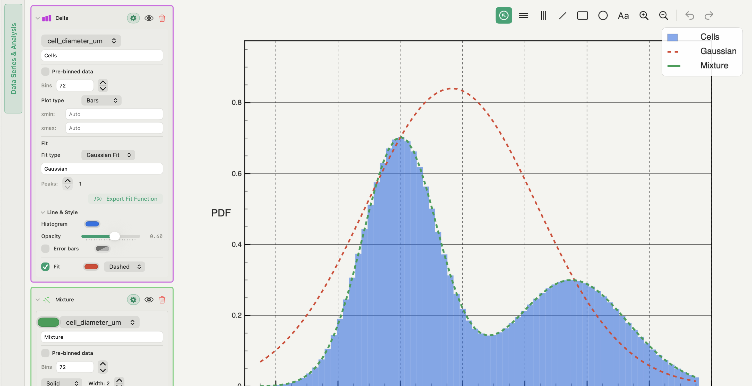
Heteroscedasticity in a residual plot
Heteroscedasticity means the error variance changes across the data. In a residuals-vs-fitted plot it appears as a funnel or a bow tie. Ordinary least squares still gives unbiased estimates for a correct model, but it gives the noisy points too much say, and the reported parameter errors are wrong.
Common remedies, in order of preference:
- Weight by known measurement errors. In SciPy's
curve_fit, pass them assigmawithabsolute_sigma=True. - Fit on a variance-stabilising scale. A log scale suits multiplicative noise, a square root suits counts, but only if the model is refitted on that scale.
- Model the variance explicitly, or use errors that are robust to heteroscedasticity, when neither of the above applies.
Histogram fits are a special case. Bin counts carry roughly Poisson noise, so the residual spread is larger where the density is high. A modest funnel under the peak is expected there and does not by itself mean the model failed.
Normality of residuals: when it matters
Least-squares estimates do not need normal errors. Confidence intervals and tests built on the t or F distribution do, especially with small samples. Look at a normal probability plot when you need those intervals, and read it after the functional form is right: a wrong model often produces skewed or heavy-tailed residuals that disappear once it is fixed.
With a few dozen points, a histogram of residuals is too coarse to judge normality. Prefer the probability plot, and do not accept or reject a model on a normality view alone.
A repeatable residual diagnostic sequence
- Keep the exact observations, fitted values, model, fit range, transforms, exclusions and weights used to compute the residuals.
- Plot residuals against fitted values with a zero line, then against every available predictor.
- If the data have an acquisition order, plot against order and against the previous residual.
- Check spread, groups, isolated points and any distributional assumption your inference needs.
- Revise the model for a scientific reason, refit, and repeat the full set.
- Report the original pattern, the change and the residuals after the change, not only the cleaner final plot.
If each added polynomial term leaves new structure behind, stop raising the degree and reconsider the model family. Starting values, bounds and convergence, which can also leave a patterned residual, are covered in nonlinear curve fitting.
Residual plots in Autoplot
The histogram fit (free plan) reports each component's amplitude, mean and sigma with parameter errors and R², and Export Fit Function turns the fitted curve into a reusable derived function. Autoplot does not draw a residual panel for you. To get one, ask the assistant to compute observed minus fitted density at the bin centres and plot it against them with a zero line; then compare a one-, two- and three-component Gaussian or your own formula on the same bins.
X&Y plots offer linear and polynomial trend overlays, but the documentation does not describe a residual output for them. For residuals of a trend or a custom model on paired data, ask the assistant: it writes the Python that fits the model and computes the residuals, shows it to you before it runs, runs it on your Mac and keeps the script, so the residual plot can be rebuilt later. Leverage, influence and autocorrelation diagnostics are not built into any card; use statsmodels or another statistics environment for those.
For the model-choice side, see how to fit a curve to data, and compare tools in curve-fitting software for Mac.
Frequently asked questions
| What does a good residual plot look like? | An even horizontal band around zero, with constant spread across fitted values and no curvature, runs or clusters. It supports the model but does not prove it. |
|---|---|
| How do I spot heteroscedasticity in a residual plot? | The vertical spread of the residuals changes with the fitted value, usually as a funnel that widens to the right. Weight the fit or change the scale before trusting the parameter errors. |
| Do residuals have to be normally distributed? | Not for the least-squares estimates themselves. Normality matters for t- and F-based confidence intervals and tests, mainly with small samples. |
Sources
Autoplot behaviour comes from the app's documentation for the histogram fit, X&Y data operations and the assistant, checked on 9 October 2026, and from the features page. The residual definition and model-adequacy framework follow the NIST/SEMATECH e-Handbook on checking model adequacy, functional-form sufficiency, a misleading fitted overlay and residuals vs fitted values, order and factors. Weighting with known errors follows the SciPy curve_fit reference.