
On this page
What makes a curve fit nonlinear
A model is linear when the prediction is a weighted sum of fixed functions of x: y = a + bx + cx², or y = a·sin(x) + b·cos(x). Least squares then has a closed-form, unique solution. A model is nonlinear when a parameter sits inside a function: a rate in an exponential, a centre or width in a Gaussian, an exponent in a power.
For nonlinear least squares, the solver (Levenberg–Marquardt or a trust-region method, as in SciPy's curve_fit and least_squares) linearises the model around the current guess, steps, and repeats. Three consequences follow: you must supply a start, the answer can depend on that start, and the reported errors come from a local linear approximation.
The broader workflow, from defining the observations to reporting, is in how to fit a curve to data. This guide covers the parts specific to the nonlinear solver.
Choosing starting values
Derive starts from the data before guessing:
- Peaks: the position of the maximum for the centre, its height for the amplitude, the half-width at half-maximum for the width.
- Decays: the plateau for the offset, the initial drop for the amplitude, the x at which the signal falls to about 37 % of its drop for τ.
- Power laws: the slope of a straight-line fit in log–log space as the first exponent.
- Composite models: fit a simpler model first and use its parameters to start the full one.
Then run a multi-start check. Draw starts across the plausible range, for example on a coarse grid or at random within the bounds, and refit from each. If different starts reach different parameter sets with similar residual sums, the data do not pin the model down; report that rather than the first answer. Keep every start in the fit record.
Parameter bounds, fixed parameters and scaling
- Bounds should encode real constraints: positive widths, fractions between 0 and 1, an instrument's range. A bound chosen to exclude an unwelcome answer turns the fit into a statement of preference.
- Estimates at a bound mean something: the model may be wrong, the parameter weakly identified, or the bound too tight. Say which, and do not quote the covariance-based error for a parameter sitting on a bound.
- Fixed parameters stabilise a fit only when the fixed value is independently known. Fixing an uncertain value hides its uncertainty in the remaining estimates.
- Scaling matters when parameters differ by orders of magnitude, say an amplitude near 10⁶ and a rate near 10⁻⁶. Rescale the model, or use the solver's scaling option (
x_scalein SciPy'sleast_squares). - Robust losses such as soft-L1 or Huber reduce the pull of outliers but change the objective. State the loss and why it suits the measurement.
Convergence checks
A solver's success flag says its stopping rule was met. It does not say the minimum is global, the model adequate or the parameters identifiable. After each fit:
- Read the termination reason. Stopping on the step-size or function-change tolerance differs from hitting the evaluation limit.
- Compare the residual sums across your multi-start runs. The best one should be reached from more than one start.
- Check that no parameter is at a bound, and that none ran to an implausible magnitude.
- Plot the residuals against fitted values, predictors and order. Structure there outranks a low cost; see how to interpret residual plots.
- Perturb the fit range and exclusions, and record which estimates survive.
Parameter uncertainty and correlation
curve_fit returns a covariance matrix from the Jacobian at the solution. The square roots of its diagonal are the usual standard errors. They assume the model is correct, the errors are independent, and the problem is close to linear near the minimum.
Two details change their meaning. If you pass known measurement errors as sigma with absolute_sigma=True, the covariance reflects those errors; with the default, it is rescaled by the residual variance. And a large off-diagonal correlation, say above 0.95 in magnitude, means two parameters trade off: the data constrain a combination, not each one. Reparameterise, collect data where the parameters separate, or report the joint uncertainty.
When the cost surface is asymmetric or the sample is small, profile the cost along each parameter or bootstrap the fit instead of quoting symmetric errors.
Nonlinear fitting checklist
- The model, parameter meanings, units and allowed ranges are written down.
- Starting values are derived from the data and recorded; a multi-start run agrees.
- Bounds, fixed parameters and weights are justified in one sentence each.
- The termination reason is read; no parameter sits at a bound unexplained.
- Residuals show no curvature, funnel or drift.
- The correlation matrix is checked; strongly coupled parameters are reported jointly.
- Estimates survive reasonable changes to range, exclusions and starts.
Nonlinear fits in Autoplot, and where to use code
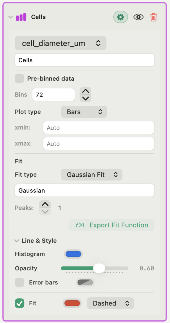
The histogram fit (free plan) is a nonlinear least-squares fit with SciPy's curve_fit on non-empty bin centres and densities. Gaussian mode fits 1–3 components with starts from the data's weighted moments, non-negative amplitudes and positive widths. Custom mode takes a predefined model (Lorentzian, exponential or uniform) or your own formula in x, plus starting guesses such as mu=10, sigma=2; unspecified parameters start at 1.0. Results include parameter errors and R².
The surface and density-map fits on heat maps (Plus) work the same way in two dimensions, with sigma-like parameters kept positive and angles kept within ±π.
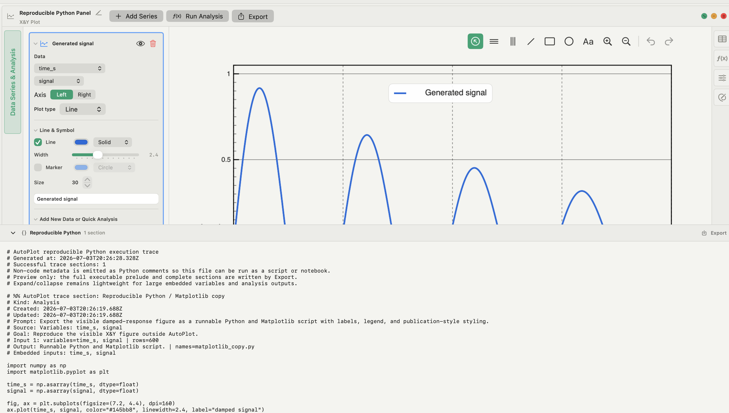
The cards do not expose user-set bounds, per-point weights, robust losses or a multi-start search, and there is no general nonlinear X/Y fitter card. For those, ask the assistant: it writes the Python (for example a least_squares fit with bounds and several starts), shows it to you before it runs, runs it on your Mac and keeps the script. Or fit in your own environment and import the results. The features page lists every fit card, and curve-fitting software for Mac compares the tools that expose bounds and weights in a GUI.
Frequently asked questions
| Why does my nonlinear fit not converge? | Usually because the starting values are far from the solution, the parameters differ in scale by orders of magnitude, or the model has more freedom than the data can constrain. Derive starts from the data, rescale, and try fixing or removing a parameter you cannot identify. |
|---|---|
| How do I choose starting values for curve_fit? | Read them off the data: peak position and height, plateau and decay length, or a log–log slope. For composite models, fit a simpler model first and use its result as the start. |
| What does it mean when a parameter ends up at its bound? | The unconstrained optimum lies outside the allowed region. Either the bound is wrong, the model is wrong, or the parameter is poorly identified; its standard error is not meaningful in that state. |
Sources
Autoplot behaviour comes from the app's documentation for the histogram fit, histogram custom fit and heat-map fits, and for the assistant, checked on 9 October 2026, and from the features page. NIST/SEMATECH describe the iterative nature, starting-value sensitivity and local-minimum risk of nonlinear least squares, give a worked approach to model selection and starting values, and note in the nonlinear regression reference datasets that solvers are not guaranteed a global minimum. Solver controls, weighting, bounds, scaling, robust losses and covariance are documented in the SciPy references for curve_fit and least_squares.