
On this page
The curve-fitting workflow in six steps
- Define the observations. Record the response, predictors, units, measurement uncertainty, exclusions, transforms and fit range. Plot the raw data first and look for impossible values, duplicates, separate groups, drift and changing spread.
- Choose the model family. Write the equation, the meaning and units of each parameter, and the domain where it should hold. Decide how errors enter: constant, proportional, or known per point.
- Estimate the parameters. Use the estimator that matches the data shape and error model, with deliberate starting values if the model is nonlinear.
- Inspect the residuals. Plot them against fitted values, each predictor and acquisition order before you interpret any parameter.
- Test sensitivity. Refit with nearby ranges, cutoffs, exclusions, bin choices and starting values. Note which conclusions move.
- Report the fit. Keep enough detail for someone else to repeat it exactly.
Keep exclusions explicit throughout. Removing an inconvenient point after seeing the result changes the analysis, and the record should say so.
Match the method to the shape of your data
The same bell-shaped picture can come from paired measurements, a histogram or a fitted surface. Decide what the estimator will actually see before you choose software or a solver.
| Data shape | Typical method | In Autoplot |
|---|---|---|
| Paired X/Y observations | Least squares: linear, polynomial or nonlinear in the parameters | Linear and polynomial trend overlays; a custom nonlinear model via the assistant or your own SciPy code |
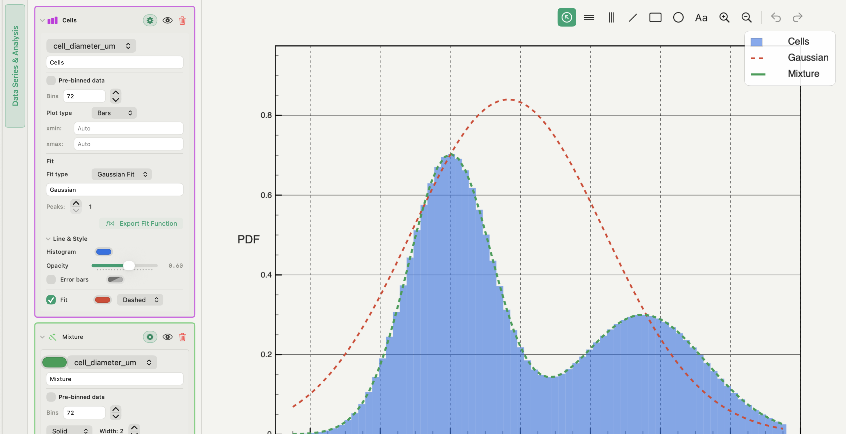
| Binned density (histogram) | Least squares on bin centres and densities, or a likelihood fit on the raw values | Histogram fit: 1–3 Gaussian components or a predefined or custom formula |
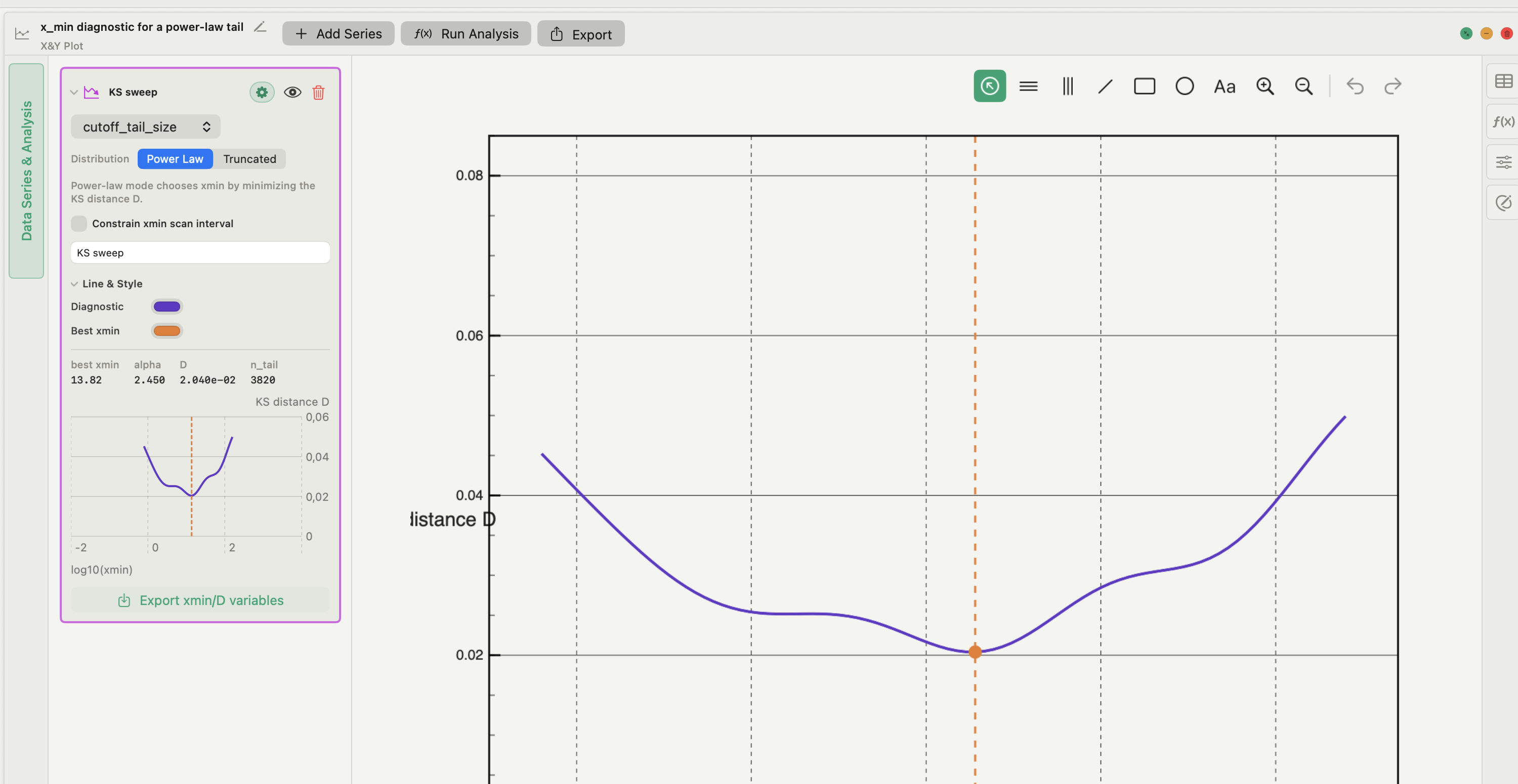
| Distribution tail | A fit above a cutoff on the raw values, read on the CCDF | CCDF tail fit and xmin diagnostic (see power-law fitting) |
| Surface z = f(x, y) or 2D density | Two-dimensional least squares | Gaussian or custom surface and density-map fits on heat maps |
A fit to bin centres depends on the bin count and range; a fit to raw observations does not. If you only have binned data, keep the original edges and normalisation with the file.
Linear vs nonlinear regression
Linear regression means the model is linear in its parameters: y = a + bx + cx² is linear, although the curve bends. Its least-squares solution is unique and needs no starting values. Nonlinear regression covers models such as y = A·e^(−x/τ) + c, where the solver searches iteratively and can stop at a local minimum.
Transforming a nonlinear model into a straight line, for example by taking logarithms, is legitimate only if the errors behave on the transformed scale. Logs turn additive noise into something else and weight small values heavily. Fit on the scale where the noise is roughly constant, or weight the points.
For a nonlinear fit, take starting values from a preliminary plot, physical expectations or a simpler model, apply bounds only where they have physical meaning, and rerun from several starts. The nonlinear curve fitting guide covers starting values, bounds, scaling and convergence in detail.
Check residuals and sensitivity before you trust the fit
A residual is the observed value minus the model's prediction. Plot residuals against fitted values, each predictor and observation order, with a zero line. Curvature means the functional form is wrong, a funnel means the variance changes, and runs in acquisition order point to drift. The guide to interpreting residual plots maps each pattern to its likely cause and the next check.
Then test the choices that could change the conclusion: the fit range, a cutoff, a baseline, the bin count, the weighting. If a parameter moves by more than its reported error when a defensible choice changes, report that sensitivity rather than one number. R² describes how closely the curve follows the points used; it neither tests the model nor compares it with alternatives.
Report the fit so someone else can repeat it
Keep and report:
- the exact input data, with every filter, transform, binning and exclusion;
- the model equation, parameterisation, units, starting values, bounds, weighting and fit range;
- the software and version, the estimator, the convergence status and the uncertainty method;
- the residual plots and the sensitivity checks that could change the conclusion;
- the editable project or script and the exact figure used.
Parameter errors from a covariance matrix assume the model and error structure are right. For consequential work, add a bootstrap or simulation check rather than relying on one asymptotic estimate.
Fitting curves in Autoplot, and where it stops
Autoplot keeps the data, the fit controls, the plot and the export in one project on your Mac.
- X&Y plots: linear and polynomial trend overlays over a chosen interval, in the free plan.
- Histogram fit: nonlinear least squares on bin centres and densities, with 1–3 Gaussian components or a predefined or custom formula with your own starting guesses. It reports the fitted parameters with errors and R², and Export Fit Function turns the curve into a reusable derived function. Free.
- Distributions: the log-binned power-law PDF fit (free), the CCDF tail fit and the xmin diagnostic (Plus).
- Surfaces: Gaussian or custom surface and density-map fits on heat maps, whose fitted surface can then be shown in a 3D plot (Plus).
There is no general nonlinear X/Y fitter card with user-set bounds and weights. For a custom model on paired data, ask the assistant: it writes the Python (typically SciPy), shows it to you before it runs, runs it on your Mac and keeps the script. You can also fit in your own environment and bring the results back as variables. See the method notes on the features page, or compare tools in curve-fitting software for Mac.
Frequently asked questions
| What is the difference between linear and nonlinear regression? | Linear regression is linear in the parameters, so polynomials count as linear and have a unique least-squares solution. Nonlinear regression has parameters inside functions such as exponentials, needs starting values and can converge to a local minimum. |
|---|---|
| Is a high R² enough to accept a curve fit? | No. R² summarises how closely the curve follows the fitted points. A wrong model can score highly while leaving systematic structure in the residuals, so inspect the residuals and test sensitivity. |
| Should I log-transform data before fitting? | Only if the noise is roughly constant on the log scale. Otherwise fit the original model directly with nonlinear least squares, or weight the points to match the measurement error. |
Sources
Autoplot behaviour comes from the app's documentation for X&Y data operations, the histogram fit and histogram custom fit, and the heat-map fits, checked on 9 October 2026, and from the features page. Model-adequacy and residual guidance follow the NIST/SEMATECH e-Handbook sections on checking model adequacy, residual analysis and a misleading fitted overlay. Nonlinear least-squares controls and covariance cautions come from the SciPy curve_fit reference.