On this page
Two methods, two kinds of input
Start from what you actually hold. Raw observations keep every value. A binned density has already compressed the sample through its edges, widths and empty-bin policy, and those choices cannot be recovered from the points alone.
| Method | Input | What is estimated | Main risk |
|---|---|---|---|
| Log-binned PDF fit | Raw values to be binned, or supplied centres and densities | Slope of log10(density) against log10(bin centre), by ordinary least squares | The exponent moves with bin count, range and dropped empty bins |
| CCDF tail fit | Positive raw observations | Tail model above xmin, fitted with the powerlaw library | A poorly chosen xmin, or too few observations in the tail |
| xmin scan | Positive raw observations | Kolmogorov–Smirnov distance D for each candidate cutoff | Treating the minimum D as proof of the model |
In Autoplot, these are three cards: the power-law and truncated power-law fit (free), the CCDF tail fit and the Xmin diagnostic (both Plus). If only pre-binned data survive, keep the original edges and normalisation with the file. Autoplot accepts supplied centres and densities, but it cannot verify how they were made.
The log-binned PDF fit: quick, and sensitive to binning
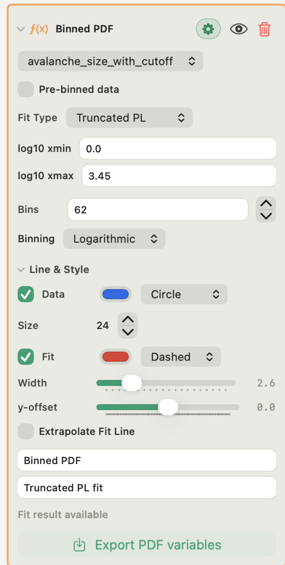
For a power-law PDF fit, Autoplot regresses log10(density) on log10(bin centre) by ordinary least squares. It reports α = −slope, an amplitude from the intercept, parameter errors and R². The truncated form, A·x^−ε·e^−λx, is fitted with SciPy's curve_fit.
That makes the estimate depend on four choices you control: the number of bins, the fitted range, the density normalisation and the removal of zero-density bins. Fit the same data with a few nearby bin counts. If α moves more than its reported error, the binning is doing some of the work.
R² measures how well a line fits the transformed, binned points. It is not the probability that the data follow a power law, and it does not compare the power law with anything else. See log binning for how the edges and densities are built.
The CCDF tail fit: raw observations above a cutoff
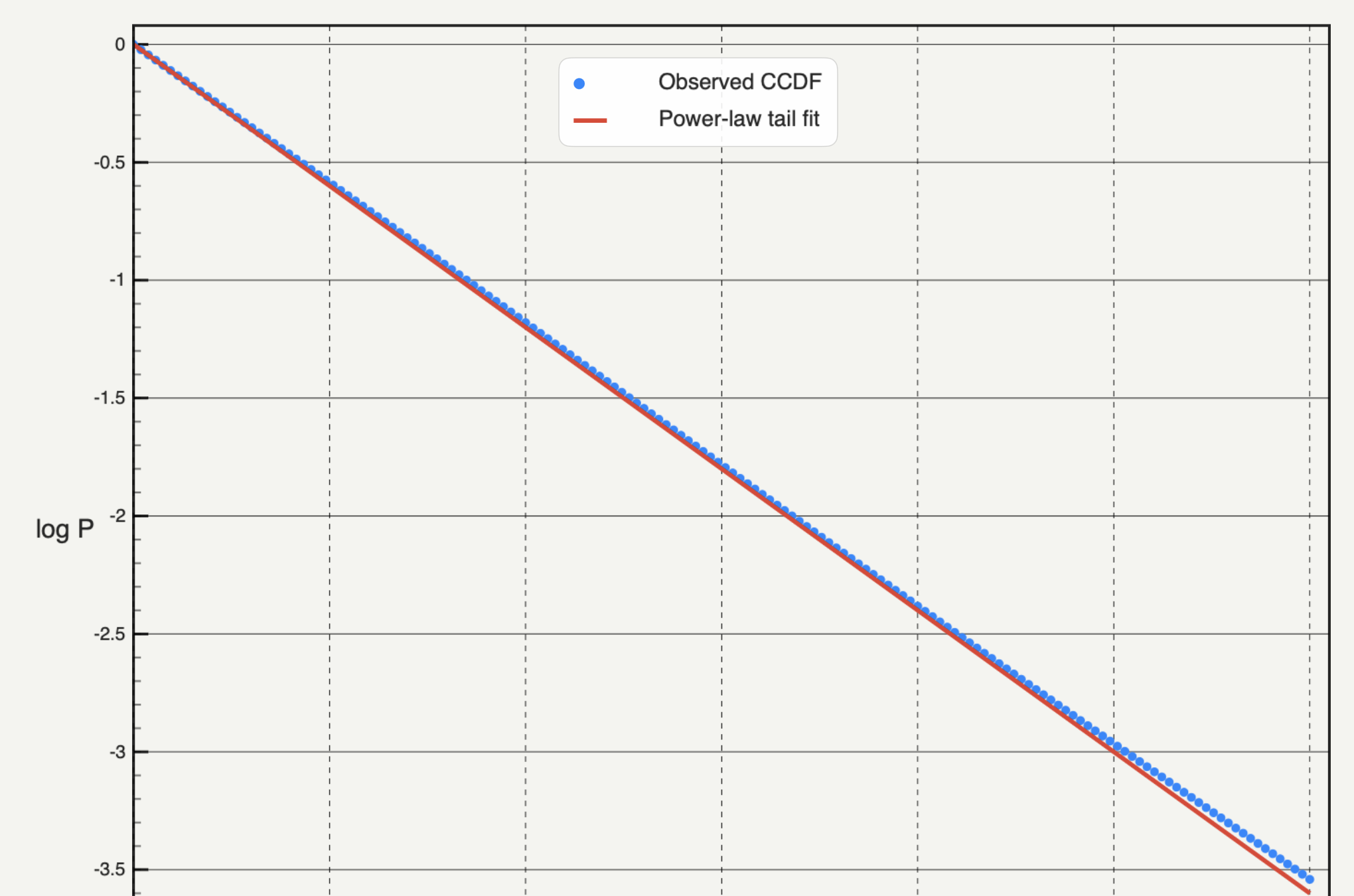
The CCDF needs no bins. Sort the positive observations and plot the share at or above each value, P(X ≥ x), on log–log axes. The tail model is then fitted from xmin upward.
In Autoplot, the CCDF card keeps values greater than zero, applies an optional xmax, and fits from the xmin you enter using the bundled powerlaw library. It offers four families: power law, truncated power law, lognormal and stretched exponential. A blank xmin means the smallest remaining positive value, not an estimated cutoff. For speed, the library fit uses a subsample of at most 1,000 observations; the empirical curve, tail count and normalisation use the full filtered sample. Report both counts.
How to choose xmin
- Plot the empirical CCDF of the positive observations before fitting anything.
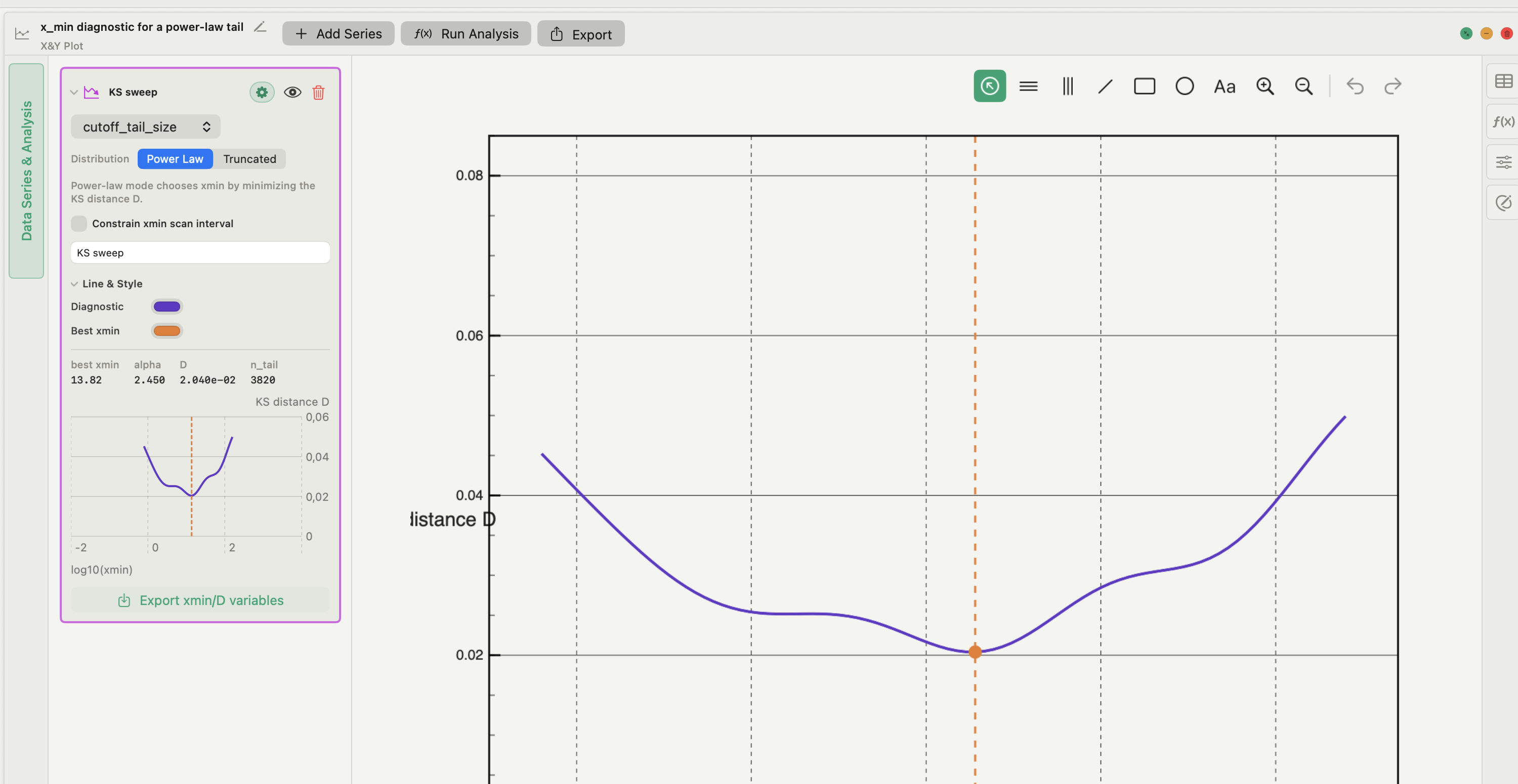
- Scan candidate cutoffs and record the Kolmogorov–Smirnov distance D between the data above each cutoff and the fitted model. Autoplot's Xmin diagnostic card runs this scan with the
powerlawlibrary on at least 50 positive values, plots D against the candidates and marks the minimum. - Take the minimum as a starting point. Refit at a few neighbouring cutoffs and check how far α and the tail count move.
- Keep enough observations in the tail. A cutoff that leaves a few dozen points can produce a stable-looking line and a meaningless exponent.
- Report xmin in natural units. Autoplot's fit fields take log10 values, so typing 3 means 1,000.
Keep the exponent convention attached
A density written as p(x) ∝ x^−α and its continuous CCDF do not share a slope. Above the cutoff, the CCDF falls as x^−(α−1). Copying a CCDF slope into a density exponent, or the reverse, shifts α by one.
State which quantity α describes, which family was fitted, the fitted range in natural units, and the number of observations in the tail. Readers cannot compare exponents without those four facts.
What a power-law claim actually needs
A straight segment on log–log axes is a reason to test, not a result. Lognormal and truncated power-law tails can look straight over two or three decades. A defensible claim usually rests on three pieces of evidence:
- Goodness of fit: a simulation-based test of whether data drawn from the fitted model resemble the observed deviations, as described by Clauset, Shalizi and Newman.
- Model comparison: likelihood-ratio comparisons against the plausible alternatives, at the same xmin.
- Sensitivity: the exponent and the comparison survive reasonable changes to xmin, xmax and, for the PDF route, the binning.
Read the CCDF plot guide to build and report the empirical tail, and PDF vs CDF vs CCDF to choose the view before you fit.
What Autoplot does, and where to go further
Autoplot keeps the data, the log-binned PDF fit, the CCDF tail fit and the xmin scan in one project on your Mac, with every range and bin choice visible on the card. The power-law PDF fit is in the free plan; the CCDF fit and the xmin diagnostic are Plus.
In Truncated mode, the Xmin diagnostic also reports the library's likelihood-ratio comparison (R and p) between a power law and a truncated power law above the chosen cutoff. The cards do not run the simulation-based goodness-of-fit test, and they do not compare against a lognormal for you. Run those in your own Python environment, or ask Autoplot's assistant to write the analysis: it writes Python, runs it on your Mac and keeps the script, so the test stays reproducible. Read the script before you rely on it. See the full method notes on the features page.
Frequently asked questions
| Is a log-log least-squares fit wrong for a power law? | Not wrong, but limited. It is a quick, transparent estimate that depends on the binning, and it gives no test of the power-law hypothesis. Use it for a first look or when only binned data exist, and say that it is a least-squares fit. |
|---|---|
| What is a good value for xmin? | The one where the data above it are best described by the model, usually found by minimising the Kolmogorov–Smirnov distance across candidates. Check that the exponent is stable around it and that enough observations remain in the tail. |
| Why do my PDF and CCDF exponents differ by about one? | Because they describe different curves. A density falling as x^−α gives a CCDF falling as x^−(α−1). Report which one you mean. |
Sources
Autoplot behaviour comes from the app's documentation for the log-space PDF fit, the log-space CCDF fit and the xmin diagnostic, checked on 9 October 2026, and from the features page. Clauset, Shalizi and Newman, Power-law distributions in empirical data, defines the xmin, goodness-of-fit and model-comparison procedure. Virkar and Clauset, Power-law distributions in binned empirical data, covers the limits binning introduces. The powerlaw package is the library behind the CCDF fit.