
On this page
How to plot a CCDF
- Define the population. Keep finite, strictly positive observations, and record how many you removed and why; zero and negative values have no place on a log axis.
- Sort the n included values in ascending order, x₍₁₎ ≤ x₍₂₎ ≤ … ≤ x₍ₙ₎.
- Assign the i-th sorted value the share of observations at or above it: P(X ≥ x₍ᵢ₎) = (n − i + 1) / n. The smallest value gets 1, the largest 1/n.
- Plot P against x with both axes logarithmic, as points rather than a joined line.
- Note n on the figure or in the caption. The lowest point is always 1/n, so the depth of the tail is set by the sample size.
In Python
After x = np.sort(x[x > 0]), the empirical CCDF is p = 1 - np.arange(len(x)) / len(x), which runs from 1 to 1/n; plot it with ax.loglog(x, p, "."). SciPy's ecdf(x).sf returns the survival function P(X > x) instead, which reaches zero at the largest value and drops that point from a log plot.
Ties and the P(X ≥ x) convention
With continuous data the convention barely matters. With repeated values it does: P(X ≥ x) and P(X > x) differ at every tie, and a ranking that gives each tied value its own step draws a short vertical run where a strict survival function would draw one point.
Rounded or integer-valued data make this visible as staircases at the low end. Decide whether to keep one point per observation or one per distinct value, and say which.

How to read a CCDF on log–log axes
Equal distances on the axes are equal ratios. The upper left of the plot holds the whole sample at P = 1; each decade down the vertical axis holds ten times fewer observations. The last decade above 1/n rests on fewer than ten values.
Neighbouring points share almost the entire sample, so the curve is smoother than the information it carries. Do not read wiggles in the lowest decade as structure, and do not judge the fit there by eye.
| What you see | What it can mean | What to check |
|---|---|---|
| A straight segment over several decades | Consistent with a power-law tail over that range | Slope is −(α−1); test against lognormal and truncated alternatives |
| A downward bend at large x | Cutoff, finite system size, or a truncated distribution | Whether the bend survives a larger sample or a different xmax |
| Gentle curvature throughout | Lognormal-like or stretched-exponential behaviour | A power-law fit to a curving CCDF depends heavily on xmin |
| Steps or plateaus | Ties, rounding or discrete values | The measurement resolution |
To decide between those readings, read how to fit a power law to data, which covers the tail fit, the choice of xmin and the evidence a claim needs. To decide whether a CCDF is the right view at all, see PDF vs CDF vs CCDF; to see the same tail as a density, build a log-binned histogram.
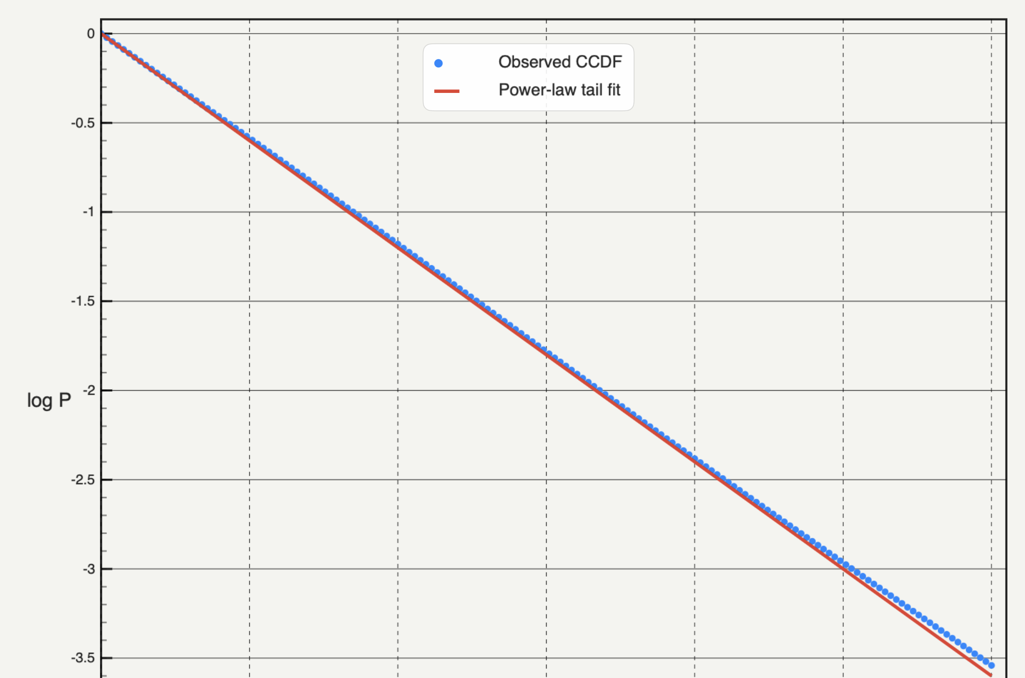
Setting the fit bounds
A tail model is fitted from a lower cutoff, xmin, upward, optionally below an upper cutoff, xmax. Both are analysis choices, not display settings.
- xmin sets where the tail begins. Leaving it at the smallest value fits the whole sample, which is rarely what a tail claim means. A Kolmogorov–Smirnov scan over candidate cutoffs gives a defensible starting point; the power-law fitting guide describes it.
- xmax removes observations above it. Use it for a known instrument limit, not to trim an inconvenient end of the tail.
- The tail count, the number of observations at or above xmin, decides how much the fit can say. A stable-looking line through a few dozen points is not a stable estimate.
Many tools, Autoplot among them, take the bounds as log10 values. Typing 3 means 1,000; report the natural value.
What to report with a CCDF plot
- Source, total count and included positive count, with the reason for every exclusion.
- The convention, P(X ≥ x) or P(X > x), and how ties were handled.
- Any xmax applied before the curve was built.
- For a fitted tail: the family, xmin and xmax in natural units, the tail count, the fitted parameters and which exponent convention they follow.
- Anything display-only, such as an offset or an extrapolated fit line.
CCDF plots in Autoplot
The Log-space CCDF card (Run Analysis, Log-Space CCDF Fit, in an X&Y figure) is part of Plus. It keeps values greater than zero, needs at least ten of them, applies an optional xmax first, and builds the empirical P(X ≥ x) from the full filtered sample with ranks from n/n down to 1/n. Tied values each keep their own point. Above 10,000 points, the stored and plotted curve is deterministically downsampled to 10,000.
The fit family is Power Law, Truncated PL, Log-Normal or Stretched Exponential, fitted with the powerlaw library on a subsample of at most 1,000 values. log₁₀ xmin and log₁₀ xmax take log10 values. A blank xmin means the smallest positive value, not an estimated cutoff, and xmin bounds the fit and the tail count without cropping the empirical points. The model line is scaled by the tail fraction so it sits on the full-sample curve; the Results block reports the exponent, the KS distance, the range and that normalisation.
The card does not export its points, and it does not run a goodness-of-fit test or a lognormal comparison. For a cutoff, run the Xmin diagnostic card; for the tests, use your own Python environment or ask the assistant to write the analysis and run it on your Mac. See the features page and pricing.
Frequently asked questions
| Should a CCDF be plotted on log–log axes? | For heavy-tailed data, yes: log–log axes spread the tail over decades and turn a power law into a straight line. For a light-tailed variable, a log vertical axis alone, or linear axes, may be clearer. |
|---|---|
| Why does my CCDF look smoother than my histogram? | Because each point accumulates all larger observations, so neighbouring points share most of their data. The smoothness is not extra information, and the lowest points remain noisy. |
Sources
Autoplot statements are based on the app's documentation for the Log-space CCDF fit and its CCDF model algorithm, checked on 9 October 2026, and the features page. SciPy's ecdf reference describes empirical CDF and survival-function estimates. Newman, Power laws, Pareto distributions and Zipf's law, explains why cumulative plots are preferred for heavy tails. Clauset, Shalizi and Newman, Power-law distributions in empirical data, sets out the fitted-range, goodness-of-fit and model-comparison requirements. The powerlaw package is the library behind the tail fit.