
On this page
PDF, CDF and CCDF compared
| View | Answers | Needs bins? | Best for |
|---|---|---|---|
| PDF (density histogram) | How concentrated are values near x? | Yes, or a kernel bandwidth | Modes, spread, shoulders, mixtures |
| CDF, P(X ≤ x) | What share is at or below x? | No | Thresholds, medians, quantiles, comparing samples |
| CCDF, P(X ≥ x) | What share is at or above x? | No | Exceedance, tail weight, heavy tails on log–log axes |
For a continuous variable the three are tied together. The CDF is the integral of the density, F(x) = ∫ f(t) dt up to x, and the density is its slope. The survival function is S(x) = 1 − F(x) = P(X > x); for continuous data P(X > x) and P(X ≥ x) coincide, and the difference only matters with ties or discrete values.
Reading a PDF
The height of a PDF is density, not the probability of one exact value. Probability is area: the integral between two values of x is the probability of landing between them. Heights carry inverse units of x and can exceed one.
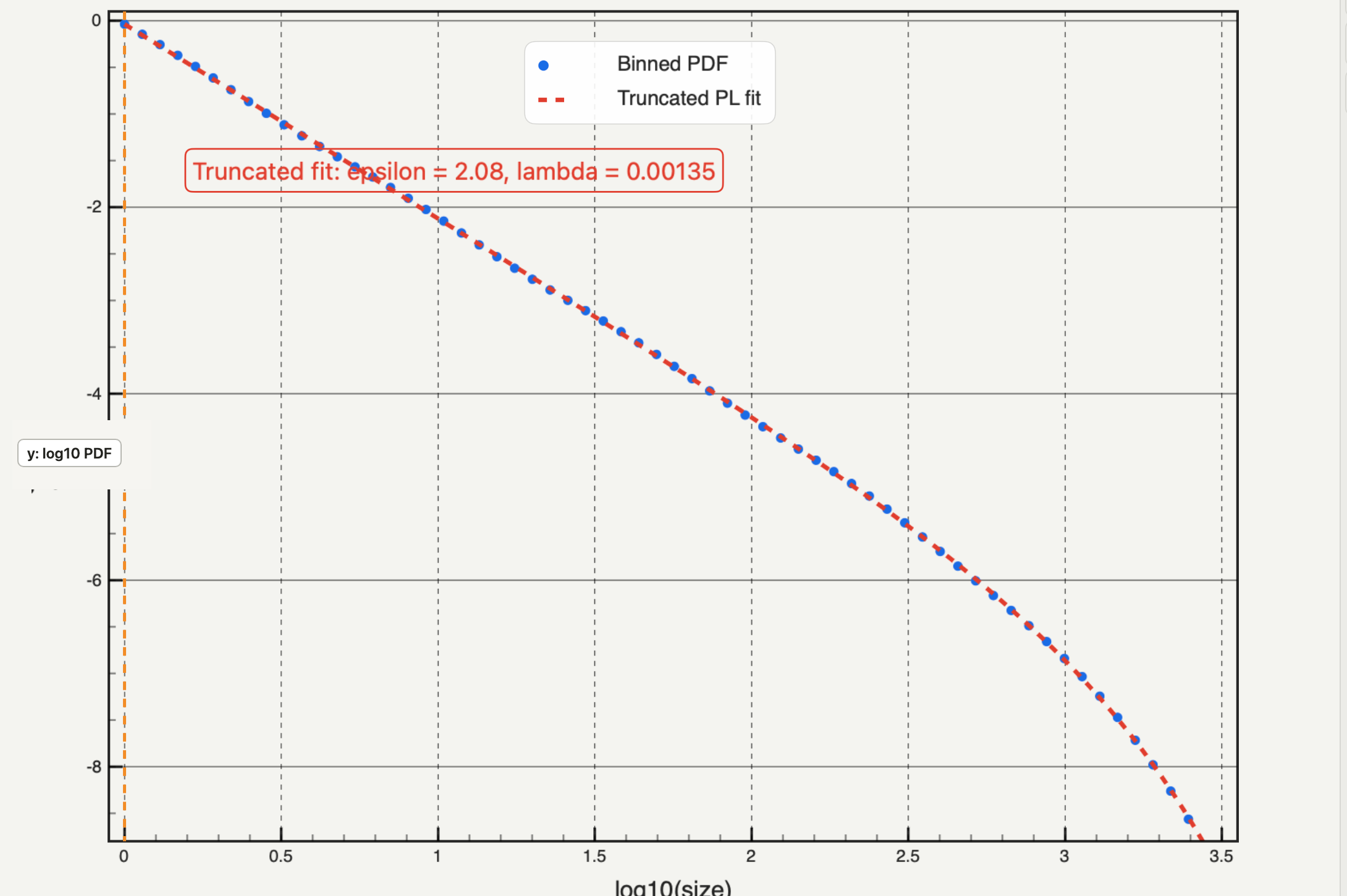
A histogram estimates the density with bins, so edges and widths shape what you see. Modes, shoulders and gaps can appear or vanish with the bin count; the histogram bin width guide sets out the check. For data across several decades, log binning keeps the density readable, provided each bin is divided by its width.
Reading a CDF
The empirical CDF sorts the observations and steps up by 1/n at each one. It needs no bins, keeps every observation's position, and answers threshold questions directly: the fraction of measurements below a tolerance, the median where F(x) = 0.5, any other quantile.
It is also the natural view for comparing samples. The Kolmogorov–Smirnov statistic is the largest vertical gap between two CDFs, which is why KS-based cutoff scans in tail fitting work on cumulative distributions.
The cost is local detail. A CDF accumulates, so a second mode shows up only as a subtle change in slope, and the upper tail is squeezed against 1, where differences of a few parts in a thousand are invisible on a linear axis.
Reading a CCDF, or survival function
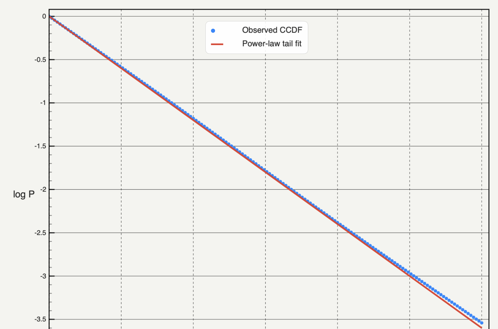
The CCDF turns the cumulative question around: what share of observations is at least this large? On log–log axes it gives the upper tail the room the CDF denies it. The smallest tail probabilities, down to 1/n, stay visible instead of being read as tiny differences from one.
Two conventions are in use. Many references, and SciPy, define the survival function as P(X > x); the empirical CCDF used for heavy-tail work is usually P(X ≥ x), so that the largest observation sits at 1/n rather than at zero, which a log axis cannot show. State which one you plot.
For a density falling as x^−α, the CCDF falls as x^−(α−1). A slope read from a CCDF is therefore not the density exponent; how to fit a power law to data keeps the two apart. Neighbouring CCDF points share most of the sample, so the curve looks smoother than the information it holds. The CCDF plot guide covers building and reading one step by step.
Which distribution view to use
Start from the sentence you intend to write.
- "Most values lie between…", "there are two populations…" Use a PDF, and check that the feature survives nearby bin counts.
- "90% of samples are below…", "the median is…" Use a CDF.
- "One event in a thousand exceeds…", "the tail decays as…" Use a CCDF on log–log axes.
- A claim about tail shape that a reviewer will question. Show the CCDF and a log-binned PDF together: a feature that appears in only one of them is suspect.
Some cases need more than a choice of view. With right-censored observations, for example survival times where some subjects were still alive at the end, the empirical CDF must be replaced by a Kaplan–Meier estimate; SciPy's ecdf handles both. Weights, truncation and range exclusions change all three views, so report them with whichever you choose.
Which views Autoplot draws
Autoplot covers the PDF and CCDF views, each with its own analysis card in an X&Y figure:
- Histogram (free): a linearly binned, density-normalised PDF in natural units, with Gaussian-mixture or custom fits. Negative values and zero are allowed.
- Log-space PDF (free): positive values only, logarithmic or linear bins, densities on log–log axes with log bins at geometric centres, with power-law, truncated power-law or custom fits.
- Log-space CCDF (Plus): the empirical P(X ≥ x) of at least ten positive values, built without bins, on log–log axes, with a tail model fitted through the
powerlawlibrary.
There is no card for an ordinary CDF, P(X ≤ x), and the CCDF card has no export button, so a CDF cannot be derived from it in the app. For an empirical CDF, use SciPy's ecdf in your own environment, or ask the assistant to write and run that Python on your Mac. The features page lists each card's inputs and outputs, and pricing shows the plans.
Frequently asked questions
| Is the CCDF the same as the survival function? | Yes, up to the convention for ties. The survival function is usually defined as P(X > x); the empirical CCDF in heavy-tail work is often P(X ≥ x). For continuous data without ties they are the same curve. |
|---|---|
| Why use a CCDF instead of a histogram for heavy tails? | A CCDF needs no bins, uses every observation, and keeps tail probabilities down to 1/n visible on log–log axes. A histogram's sparse tail bins are noisy and depend on the bin choice. |
| How do you get the PDF from the CDF? | The PDF is the derivative of the CDF. For data, differentiating the empirical CDF is noisy, so the density is estimated directly with a histogram or a kernel instead. |
Sources
Autoplot statements are based on the app's documentation for the Histogram, Log-space PDF and Log-space CCDF cards and the CCDF model algorithm, checked on 9 October 2026, plus the features page. The NIST/SEMATECH handbook's related distributions page defines the density, cumulative distribution and survival functions. SciPy's ecdf reference covers empirical CDF and survival estimates, including censored data. NumPy's histogram reference defines the binned density. Newman, Power laws, Pareto distributions and Zipf's law, and Clauset, Shalizi and Newman, Power-law distributions in empirical data, explain why cumulative views are preferred for heavy tails and what a tail claim requires.