On this page
Freedman–Diaconis, Scott's rule and Sturges compared
Most rules give a bin width h; the number of bins follows as k = ⌈(max − min) / h⌉ over the range you fix. Here n is the number of included observations, IQR the interquartile range and σ the sample standard deviation.
| Rule | Width or count | Good for | Caveat |
|---|---|---|---|
| Freedman–Diaconis | h = 2 · IQR · n^(−1/3) | Skewed data, outliers | Many bins when a long tail stretches the range; fails when ties make the IQR zero |
| Scott's rule | h = 3.49 · σ · n^(−1/3) | Roughly normal data | Outliers inflate σ and widen every bin |
| Sturges' rule | k = ⌈log2(n)⌉ + 1 | Small, near-normal samples | Too few bins for large or non-normal samples |
| Square root | k = ⌈√n⌉ | A quick first look | Ignores spread and shape |
NumPy's bins="auto" takes the smaller width of Sturges and Freedman–Diaconis, which in practice means Sturges for small samples and Freedman–Diaconis for large ones. It is a sensible default, and it still knows nothing about the scientific meaning of a feature.
How many bins should a histogram have
As many as the data can support around the structure you care about, and no more. A useful procedure:
- Decide which observations belong in the histogram. Remove non-finite values, record scientific exclusions and say whether out-of-range values were excluded or merely hidden.
- Fix the range. Changing it changes the represented population and the width of every equal-width bin.
- Compute a starting width with one of the rules above and convert it to a bin count for that range.
- Render at least one coarser and one finer version, for example half and double the count, on the same range.
- Shift the edges by a fraction of a bin. A narrow cluster can be split by an edge in one view and sit inside one bar in the next.
- Keep the conclusions that survive steps 4 and 5, and freeze the final edges before fitting anything to the bars.
The measurement's resolution is a floor. Bins narrower than the instrument can resolve, or than a rounding step in the data, produce combs and empty intervals that describe the recording, not the variable.
What a bin-width sensitivity check should look for
Compare the views for the features you intend to report, not for overall smoothness.
- Modes: a second peak that appears at only one bin count, or vanishes with a small edge shift, is not yet a result.
- Gaps and shoulders: a gap that persists across counts may be real; one that appears only with narrow bins is often sampling noise.
- Skew and tails: wide bins compress a tail into one or two bars. If the tail is the question, read log binning or use a cumulative view from PDF vs CDF vs CCDF, which needs no bins at all.
Very wide bins hide variation; very narrow bins amplify noise. When a feature survives only in a narrow window of choices, inspect the raw observations before describing it.
Comparing groups
Compute one range and one edge array for all groups. Two histograms with separate automatic ranges can have the same bin count and still cover different intervals, so equal-looking bars are not comparable. If the groups differ in size, compare proportions or densities rather than counts; the histogram normalization guide sets out which.
Bin width changes the fit as well as the picture
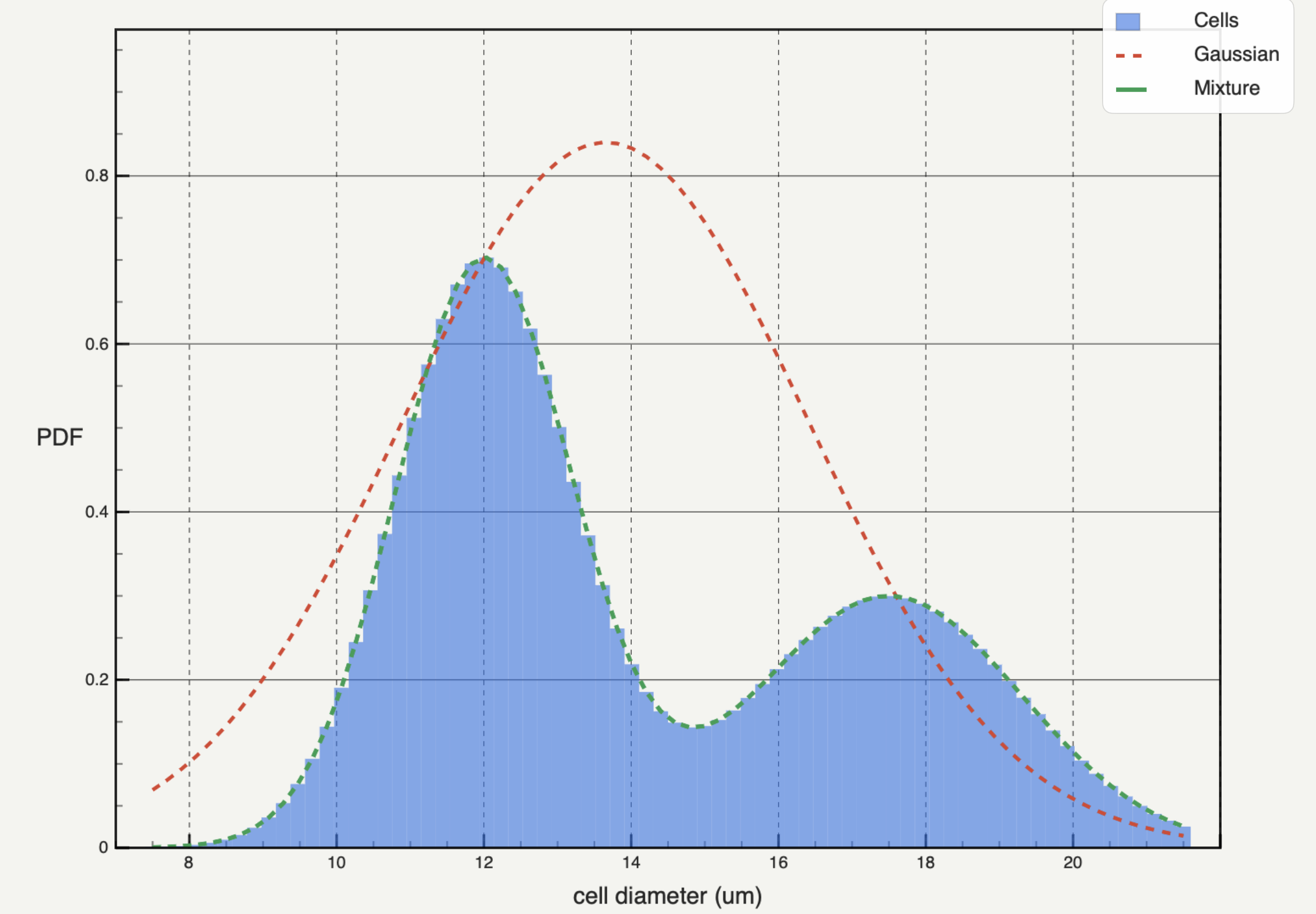
A curve fitted to a histogram is fitted to the bin centres and heights, not to the observations. Changing the bin count or the range changes those points, so it can change the fitted parameters and their errors.
Refit at the neighbouring bin counts from your sensitivity check. If a parameter moves by more than its reported error, the binning is part of the estimate and should be reported as such. For the model-checking side, see how to fit a curve to data and how to interpret residual plots.
What to report
- Source variable, units and the number of included observations.
- Exclusions: non-finite values, scientific filters and the range limits.
- The rule used as a starting point, the final bin count and the width, or the full edge array if bins are unequal.
- The normalisation of the vertical axis.
- For a fitted histogram: the fit settings, and the number of non-empty bins that entered the fit.
Choosing bins in Autoplot
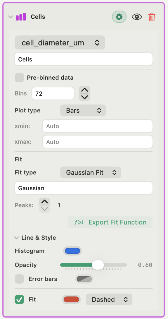
The Histogram card (Run Analysis, Histogram Fit, in an X&Y figure) is in the free plan. It takes a Bins value, clamped to 1–1000, and natural-value xmin and xmax fields; left empty, they use the data minimum and maximum. Edges are linearly spaced across that range, heights are always density-normalised, and centres are arithmetic midpoints. Negative values and zero are allowed.
Empty bins are drawn but do not enter the Gaussian-mixture or custom fit, which needs at least three non-empty bins per Gaussian component. Because bins and range stay on the card, a sensitivity check is a matter of changing one field and refitting.
Autoplot does not compute Freedman–Diaconis, Scott or Sturges for you. Compute the width with NumPy's histogram_bin_edges, or ask the assistant, which writes and runs the Python on your Mac, then type the resulting count into Bins with the range fixed. For bins of unequal width, positive data across decades use the log-binned PDF card instead; see the features page.
Frequently asked questions
| How many bins should a histogram have? | There is no single answer. Start from Freedman–Diaconis or Scott's rule for your range, then check that the features you report survive half and double that count. |
|---|---|
| Is Freedman–Diaconis better than Sturges' rule? | For large or skewed samples, usually yes. Sturges depends only on sample size and gives too few bins as n grows; Freedman–Diaconis scales with the interquartile range and resists outliers. |
| Should two histograms I compare use the same bins? | Yes. Use one range and one set of edges for both, otherwise the bars cover different intervals and cannot be compared directly. |
Sources
Autoplot statements are based on the app's documentation for the Histogram card and its binning, checked on 9 October 2026, and the features page. NumPy's histogram_bin_edges reference gives the estimator formulas, the auto rule and their limits; its histogram reference defines edges and density. The NIST/SEMATECH handbook's histogram page describes the histogram as a summary of a univariate distribution whose classes are set by the user or by a rule.