On this page
When to use logarithmic binning
Linear bins ask what happens in equal additive intervals; logarithmic bins ask what happens in equal multiplicative ones. Use log bins when the data are strictly positive, span at least two or three orders of magnitude, and the question concerns the shape of a broad or heavy-tailed distribution.
| Property | Linear bins | Logarithmic bins |
|---|---|---|
| Bin width | Constant | Grows in proportion to x |
| Plotted position | Arithmetic midpoint | Geometric centre |
| Tail bins | Mostly empty, or one wide bar | Spread evenly per decade |
| Zero and negative values | Allowed | Excluded; record why |
If the question is only about the upper tail, an empirical CCDF avoids binning altogether. PDF vs CDF vs CCDF sets out when each view fits, and the CCDF plot guide shows how to build one.
How to log-bin data
- Keep finite, strictly positive observations. Zero and negative values have no position on a log axis; count and report what you removed.
- Fix the range, usually the smallest and largest retained values, and choose a bin count k. Reporting bins per decade makes the choice comparable between datasets.
- Build k + 1 edges spaced by a constant ratio: eⱼ = xmin · (xmax / xmin)^(j/k).
- Count the observations in each bin.
- Convert to density: divide each count by the total n and by that bin's width, eⱼ₊₁ − eⱼ.
- Place each point at the geometric centre, √(eⱼ · eⱼ₊₁).
- Plot density against centre on log–log axes, and note which bins were empty.
Log bins in Python
Build the edges with np.logspace(np.log10(x.min()), np.log10(x.max()), k + 1), or equivalently np.geomspace(x.min(), x.max(), k + 1). Then np.histogram(x, bins=edges, density=True) divides by each bin's own width, so unequal widths are handled. Compute centres as np.sqrt(edges[:-1] * edges[1:]) and keep the empty bins in a separate array before you mask them for the log–log plot.
Why width normalisation and geometric centres matter
With logarithmic edges, a bin at x = 1,000 is a thousand times wider than one at x = 1. Plotting raw counts would let the wide tail bins collect observations simply because they cover more of x, flattening the apparent decay. Dividing by width turns each bar into probability per unit of x, so the area, density × width, is the probability of the interval. The histogram normalization guide covers the denominators in general.
An arithmetic midpoint sits to the right of the centre of a log bin, and the offset grows with the bin's ratio. On a log–log plot that shifts every point along the x axis and bends a slope estimated from the points. The geometric centre is the midpoint in log space and is the standard choice.
Density keeps units. If x is in seconds, density is per second, even when both axes show log10 values.
Empty bins and the choice of bin count
An empty bin means no included observation fell in that interval. Its density is zero, and log(0) is undefined, so log–log plots usually drop it. That is acceptable for display, but it hides how sparse the tail is and lets a fitted line pass only through the populated bins. Keep the full edge array and the empty-bin count alongside the plotted points.
Sparse tail bins have a second problem: a bin holding one or two observations gives a density with very large relative error. Too many bins produce a ragged, gappy tail; too few smooth away a genuine bend.
Compare a few nearby bin counts on the same range. Broad structure should persist. A shoulder, kink or slope that moves with the count is a property of the binning and should not be reported as a property of the data.
A straight log-binned PDF is not yet a power law
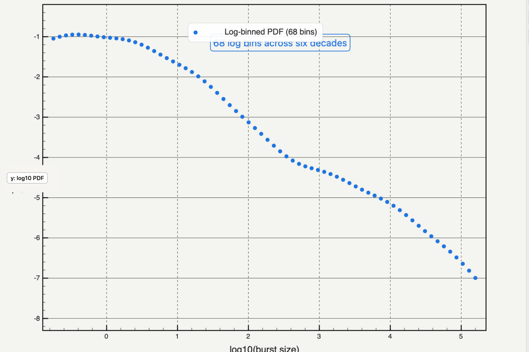
Range, bin count, sparse tail bins and dropped empty bins can all create or straighten a linear-looking segment on log–log axes. Lognormal and truncated distributions can look straight over two or three decades. Fitting and testing are a separate step: how to fit a power law to data covers the least-squares fit on the binned PDF, the CCDF alternative and the evidence a power-law claim needs.
Log binning in Autoplot
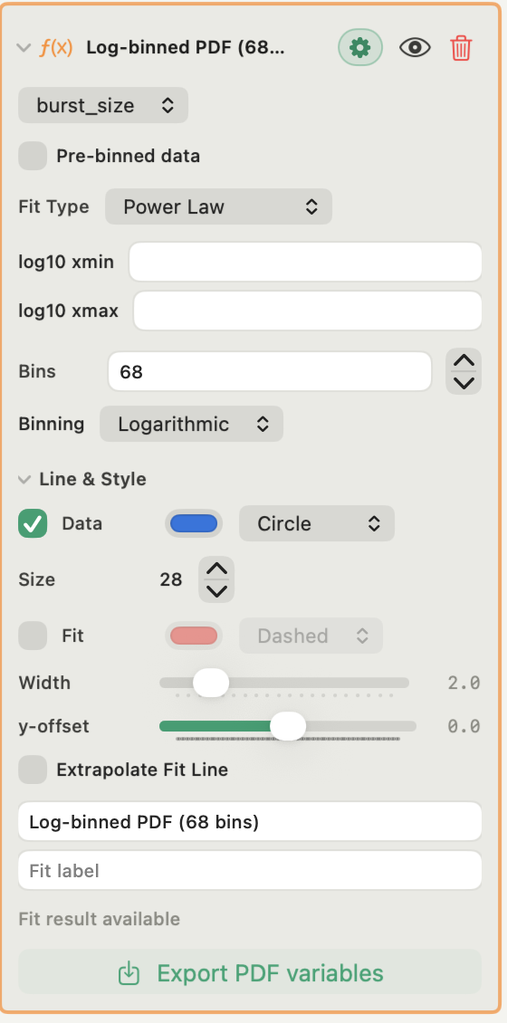
The Log-space PDF card (Run Analysis, Log-Space PDF Fit, in an X&Y figure) is in the free plan. From raw observations it keeps values greater than zero and builds edges from the smallest to the largest positive value. Binning defaults to Logarithmic, with Linear available; Bins defaults to 50 and is clamped to 1–1000.
Densities come from NumPy's density=True. Logarithmic bins are plotted at geometric centres, linear bins at arithmetic midpoints, and zero-density bins are removed from both the plotted and the fitted points. The log₁₀ xmin and log₁₀ xmax fields bound the fit only, in log10 units: typing 2 means 100. There is no separate control for the bin range.
Export PDF variables writes the bin centres, densities, bin widths and the fit line as variables, so the binned PDF can be reused or checked. With Pre-binned data, the card accepts centres and densities you supply, but it cannot verify their widths or empty-bin policy. The features page lists the fit families.
Frequently asked questions
| Why divide a log-binned histogram by bin width? | Because log bins widen with x. Without the division, wide tail bins collect observations because they are wide, and the plotted decay is too shallow. |
|---|---|
| Should I use log binning or a CCDF? | Use log binning when you need a density, for example to see a peak or to fit a binned PDF. Use a CCDF when the question is about the tail and you have the raw observations, since it needs no bins. |
Sources
Autoplot statements are based on the app's documentation for the Log-space PDF fit and its binning and density algorithm, checked on 9 October 2026, and the features page. NumPy's histogram reference defines non-uniform edges and width-aware density, and its geomspace reference covers ratio-spaced edges. Newman, Power laws, Pareto distributions and Zipf's law, discusses logarithmic binning and the cumulative alternative. Clauset, Shalizi and Newman, Power-law distributions in empirical data, explains why a straight log–log line does not establish a power law.