
On this page
- Why overlapping peaks need joint deconvolution
- Choosing Gaussian, Lorentzian, Voigt, or mixed shapes
- Detection, baselines, and center locking
- Reading residuals, AIC/BIC, and failure modes
- Native Mac alternative to Igor Pro and MagicPlot Pro for peak fitting
- Peak Deconvolution in Autoplot
- Frequently asked questions
Why overlapping peaks need joint deconvolution
In an additive 1D spectrum or trace, the measured signal at coordinate combines an underlying background and individual peak profiles:
Integrating raw intensity above a straight chord or fitting each maximum in a narrow sub-window works only when neighboring peaks sit many full widths apart. Once tails overlap—as in doublets, unresolved shoulders, or bands resting on fluorescence or thermal drift—clipping windows biases peak heights upward or downward, narrows apparent FWHM, and shifts peak centers toward the taller neighbor. At the same time, joint fits are not automatically unique: Maddams (1980) notes that unresolved shoulders and floating baselines easily trade off unless component count, line shape, or known band centers are physically constrained.
If your spectrum shows negative absorption dips rather than positive emission peaks, set the fit polarity before detecting candidates so both the baseline estimate and peak amplitudes carry consistent signs. For general model formulation before choosing a line shape, start with how to fit a curve to data.
Choosing Gaussian, Lorentzian, Voigt, or mixed shapes
Each peak profile parameterizes position by center , integrated area , and intrinsic width parameters that determine both apex height and full width at half maximum (FWHM):
| Shape | Broadening mechanism | Parameterization and FWHM | Watch out for |
|---|---|---|---|
Gaussian | Inhomogeneous broadening, Doppler spread, or Gaussian spectrometer slit | Area , center , width ; | Decays too quickly in the wings; leaves negative/positive wing errors on lifetime-broadened peaks |
Lorentzian | Homogeneous relaxation or finite excited-state lifetime | Area , center , half-width ; | Heavy wings borrow intensity from the baseline if bounds are loose |
Voigt | Convolved Gaussian core and Lorentzian tails | Exact Faddeeva evaluation over with mixing | Adds two shape parameters per peak; needs enough points and distinct wings to separate from |
Mixed | Heterogeneous spectrum (e.g., sharp reference spike beside broad band) | Independent G, L, or V shape per seed solved simultaneously | Increases model combinations; keep physical justification for each peak's assigned profile |
In Autoplot, the Gaussian component takes , the Lorentzian component takes , and the Voigt profile evaluates at , using the Olivero and Longbothum (1977) linewidth approximation to seed an exact numerical FWHM root.
Detection, baselines, and center locking
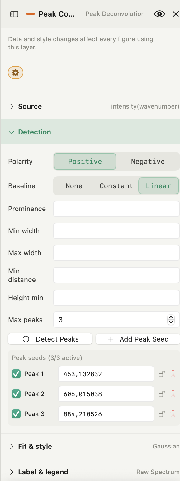
Multi-peak nonlinear least squares is non-convex, so two poorly placed seeds can swap positions, collapse onto one wide band, or pull a flat baseline upward. A structured five-step setup keeps the optimization stable:
- Restrict the fit window only where the model holds: set
Fit X minandFit X maxto frame the spectral region of interest, leaving enough flank points outside the outer peaks to constrain the baseline slope without dragging in unrelated bands. - Choose the simplest defensible baseline (
None,Constant, orLinear): useConstantfor a flat dark-count floor andLinearfor slow fluorescence or thermal drift across the window. Autoplot initializes linear baselines from outer edge percentiles and asymmetric iteratively reweighted least squares (IRLS) so bright peaks do not pull the initial floor upward. - Run prominence-based detection, then inspect every seed: when
Prominenceis left blank, Autoplot estimates high-frequency noise from second differences and sets a noise-scaled threshold before callingscipy.signal.find_peaks. IncreaseMin width,Min distance, orMax peaksto reject noise spikes, or click+ Add Peak Seedto mark an unresolved shoulder the maximum-finder missed. - Lock known peak positions when shoulders trade off: if two adjacent centers slide toward each other or produce huge parameter errors, lock a known reference line position (
x₀) while keeping weaker neighbors free. The trade-offs around starting guesses, bounds, and collinear parameters are covered in nonlinear curve fitting. - Run the joint solver and check parameter uncertainties: Autoplot optimizes all active peaks and baseline coefficients together with bounded Trust Region Reflective least squares (
trf), then scales the Gauss–Newton pseudoinverse covariance by reduced chi-squared to report±standard errors on centers, widths, areas, apex heights, and baseline terms.
Reading residuals, AIC/BIC, and failure modes
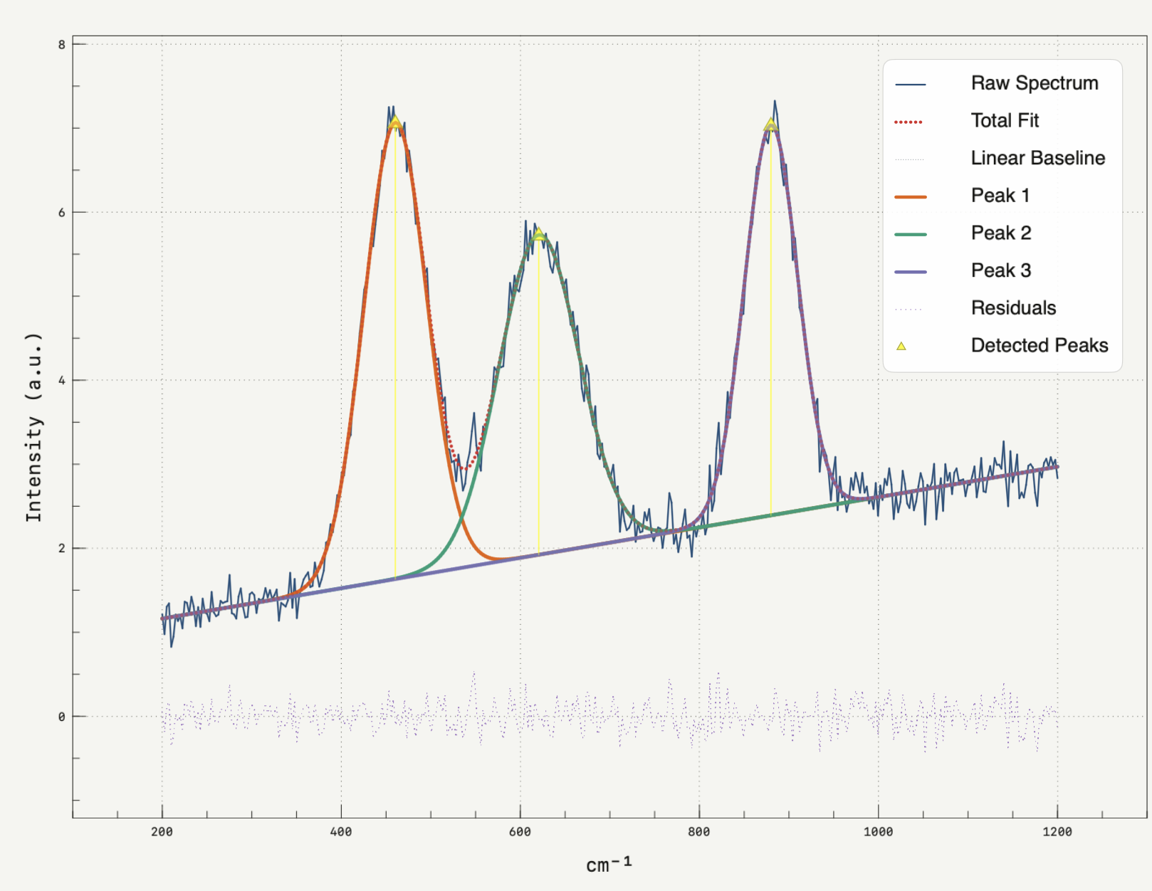
High is easy to achieve across three peaks and reveals little about whether you chose the right number of components or line shape; as Major et al. (2020) show for X-ray photoelectron spectroscopy (XPS), adding unconstrained peaks lowers the raw residual sum while still producing unphysical widths and chemical-state assignments. Check four diagnostics under Results and on the plot:
- Residual trace patterns: toggle
Residualson. Random noise centered on zero indicates a consistent additive model; an S-shaped dipole or positive bump sitting directly under a flank points to an omitted shoulder seed, while symmetric negative wings beside a sharp core usually signal thatGaussiantails decay too fast and needLorentzianorVoigt. See how to interpret residual plots for reading systematic patterns. - Model comparison via
AICandBIC: keep the exact same[Fit X min, Fit X max]dataset window when comparingGaussianvsVoigtor3vs4peaks. Because adding parameters always lowersRMSE, a meaningful improvement lowersAICandBICrather than inflating parameter standard errors. - Width-bound warnings: if a component width expands until it touches the upper bound (
2 × span), that peak is usually acting as a surrogate curved baseline. SwitchBaselinefromNonetoConstantorLinear, narrow out unrelated continuum drift, or lock a constrained seed center. - Duplicate centers and tiny slices: putting two unlocked seeds of identical shape at the same
x₀creates collinear columns in the Jacobian, and slicing[Fit X min, Fit X max]below the total free parameter count fails validation. Keep several points per FWHM across every fitted peak.
Native Mac alternative to Igor Pro and MagicPlot Pro for peak fitting
If you previously relied on Igor Pro or MagicPlot Pro solely to deconvolve spectra on a Mac, the decision now splits by platform and constraint depth:
| Need | Autoplot | Igor Pro | MagicPlot / MagicPlot Pro |
|---|---|---|---|
| Mac platform | Native Apple silicon (macOS 15+) | 9.05 Intel under Rosetta 2; 10 is Windows-only | Native Apple silicon and Intel builds (3.2) |
| Peak and baseline models | Gaussian, Lorentzian, Voigt, mixed; none, constant, or linear baselines | Built-in and user-defined multipeak and baseline models | Multipeak Gaussian, Lorentzian, Voigt, and baseline curves |
| Parameter control | Lock individual centers (x₀); unweighted least squares | Constrained, coupled, global linked fits, and weighted least squares | Locked or joined parameters, weighted by Y errors, batch tables |
| Native files and handoff | CSV/text import; peak tables, curves, and Python out | Opens .pxp and .ibw; built-in procedure language | Opens .mppz; EPS, PDF, SVG, and EMF vector export |
For routine single-spectrum multi-peak fitting from CSV or delimited text—especially if you are moving off Intel-only Igor Pro 9.05 without booting Windows—Autoplot handles peak finding, baseline fitting, component curves, AIC/BIC comparison, and multi-panel composition natively on Apple silicon. Keep Igor Pro when a workflow depends on global linked fits, acquisition XOPs, procedure files, or .pxp/.ibw experiments, and keep MagicPlot when you need .mppz project compatibility, coupled parameters, Y-error weights, or batch-series parameter summaries.
Peak Deconvolution in Autoplot
Autoplot's Peak Deconvolution analysis (Run Analysis → Peak Deconvolution in any X&Y Plot, Plus — free for 30 days) runs candidate peak finding and joint multi-peak optimization locally on your Mac:
- Inputs (
Source&Detection): selectYand optionalX (opt.)(defaulting to row index when omitted), restrict[Fit X min, Fit X max]if needed, choosePositiveorNegativepolarity andNone/Constant/Linearbaseline, adjust optionalProminence,Min width,Max width,Min distance,Height min, andMax peaks, then clickDetect Peaksor+ Add Peak Seedand toggle per-seed enable/lock states. - Model & overlays (
Fit & style): switch globally betweenGaussian,Lorentzian,Voigt, or per-seedMixedshapes, toggleShow fit,Baseline,Components,Comp + base(adds the baseline under each component),Peak pins, andResiduals, customize line colors, strokes, markers, andY offset, then click the orange gear button (Fit peaks/Refit peaks). - Results & exports (
Figure Inspector → Results): inspectPeaks,R²,Adj R²,RMSE,AIC,BIC,χ²_red,DOF, baselineb₀ ± stderr/b₁ ± stderr, and the per-peak table (#,Shape,Center,Height,FWHM,Area,%), then export viaExport Peak TableorExport Deconvolved Curves(curveX,totalFitY,baselineY, and component curves asDerived Variables). You can also set up and trigger deconvolution layers from the AI Assistant in Execute mode without sending raw numerical array values off your Mac. - Where it stops: optimization uses unweighted ordinary least squares over additive symmetric
Gaussian,Lorentzian, andVoigtprofiles; asymmetric Fano profiles, non-polynomial spline baselines, parameter inequality coupling across peaks, and per-point error weighting (σ_y) are not built into the card—use a custom SciPy workflow when those are required.
Frequently asked questions
| When should I choose Voigt instead of Gaussian or Lorentzian? | Use Gaussian when broadening comes mainly from spectrometer resolution, thermal Doppler spread, or random inhomogeneity, and Lorentzian when natural lifetime broadening creates wide tails. Choose Voigt when both mechanisms contribute comparably, then verify that AIC and BIC improve without huge uncertainties on σ or γ. |
|---|---|
| Should I subtract a linear baseline before fitting overlapping peaks? | No—keep Baseline set to Constant or Linear inside the deconvolution fit. Pre-subtracting a hand-drawn line ignores how baseline slope trades off against overlapping peak tails, whereas joint fitting estimates baseline b₀ and b₁ together with peak widths and propagates their covariance into peak areas. |
| What does locking a peak seed center do? | Clicking the lock toggle on a seed removes that peak's center μ from the free parameter vector while keeping its amplitude and width parameters free. Use locking when an overlapping satellite shares the flank of a well-calibrated reference line whose position is known independently. |
| Does Autoplot support weighted least squares or asymmetric peak shapes in Peak Deconvolution? | Not inside the Peak Deconvolution card: the solver runs unweighted Trust Region Reflective least squares over additive symmetric Gaussian, Lorentzian, and Voigt components with optional constant or linear baselines. For Y-error weighting or asymmetric Fano lineshapes, export your variables or run a custom SciPy least_squares script. |
| Can Autoplot replace Igor Pro or MagicPlot Pro for multi-peak fitting on a Mac? | For single-spectrum overlapping Gaussian, Lorentzian, Voigt, or mixed peaks from CSV or text files, Autoplot replaces that workflow natively on Apple silicon without Rosetta 2 or Windows virtualization. Keep Igor Pro for global linked fits, procedures, and .pxp/.ibw files, and keep MagicPlot Pro for .mppz projects, coupled parameters, Y-error weights, or batch-series peak tables. |
Sources
Algorithm details (detect_peaks_1d, asymmetric IRLS baseline initialization, bounded trf fit_multipeak_deconvolution, Faddeeva wofz Voigt evaluation, brentq Voigt FWHM solver, Gauss–Newton pseudoinverse covariance propagation, AIC/BIC, and χ²_red) and UI labels (Peak Deconvolution, Detection, Peak seeds, Fit & style, Comp + base, Peak pins, Residuals, Export Peak Table, Export Deconvolved Curves) were verified directly against Autoplot 2.3.0 / 2.4.0 source (math_logic.py, PeakDeconvolutionResultsView.swift, and Autoplot's Peak Deconvolution documentation) on 22 November 2026. Underlying numerical routines use SciPy's `find_peaks`, `least_squares`, and Faddeeva `wofz`. Overlapping-band uniqueness and baseline trade-offs draw on W. F. Maddams, "The Scope and Limitations of Curve Fitting," *Applied Spectroscopy* 34(3), 245–267 (1980), DOI `10.1366/0003702804730312`; practical XPS peak-fitting constraints and residual diagnostics draw on G. H. Major, N. Fairley, P. M. A. Sherwood, M. R. Linford, J. Terry, V. Fernandez, and K. Artyushkova, "Practical guide for curve fitting in x-ray photoelectron spectroscopy," *Journal of Vacuum Science & Technology A* 38(6), 061203 (2020), DOI `10.1116/6.0000377`; and Voigt half-maximum linewidth initialization draws on J. J. Olivero and R. L. Longbothum, "Empirical fits to the Voigt line width: A brief review," *Journal of Quantitative Spectroscopy and Radiative Transfer* 17(2), 233–236 (1977), DOI `10.1016/0022-4073(77)90161-3`90161-3).