
On this page
MagicPlot vs Autoplot: side by side
| Need | MagicPlot | Autoplot |
|---|---|---|
| Mac support | Native Apple silicon and Intel builds | Apple silicon only, macOS 15 or later |
| Project structure | .mppz with Tables, Figures and Fit Plots | .elab with variables, figures and analysis layers |
| Nonlinear X/Y fitting | Fit Plots with predefined or custom equations | No general fitter; linear and polynomial trends on X&Y |
| Multipeak and baseline | Interactive, with guessed peaks and baseline subtraction | Not available |
| Batch work | Batch fitting with a parameter summary table | Batch import and variable creation; no batch figure export |
| Plot types | 2D figures; vector export to EPS, PDF, SVG and EMF | 2D, heat maps and 3D; PNG, JPEG and vector PDF |
Opens .mppz | Yes | No |
MagicPlot is a fitting tool that draws good figures. Autoplot is a data-to-figure tool with specialist analysis cards. If you are reading this because of the fitting, the table already answers the question.
Where MagicPlot is the better choice
Keep MagicPlot when the work is any of these:
- Spectra or patterns with overlapping peaks. Building a model peak by peak, dragging each into place with the mouse and fitting the sum is exactly what a Fit Plot is for.
- Baseline-corrected data. Baseline curves are fitted and subtracted inside the same Fit Plot, with the corrected data kept as a column.
- Constrained models. Lock a parameter so it cannot move, or join parameters across curves so they share a value.
- Weighted fits. With Y errors supplied, each point is weighted by the inverse square of its error.
- Many similar datasets. Batch processing fits a series the same way and collects the parameters in one table.
MagicPlot also notes that its fitter was tested on the NIST nonlinear regression datasets. For the general method, see the nonlinear curve fitting guide.
Autoplot as a MagicPlot alternative for new projects
Distributions rather than peaks
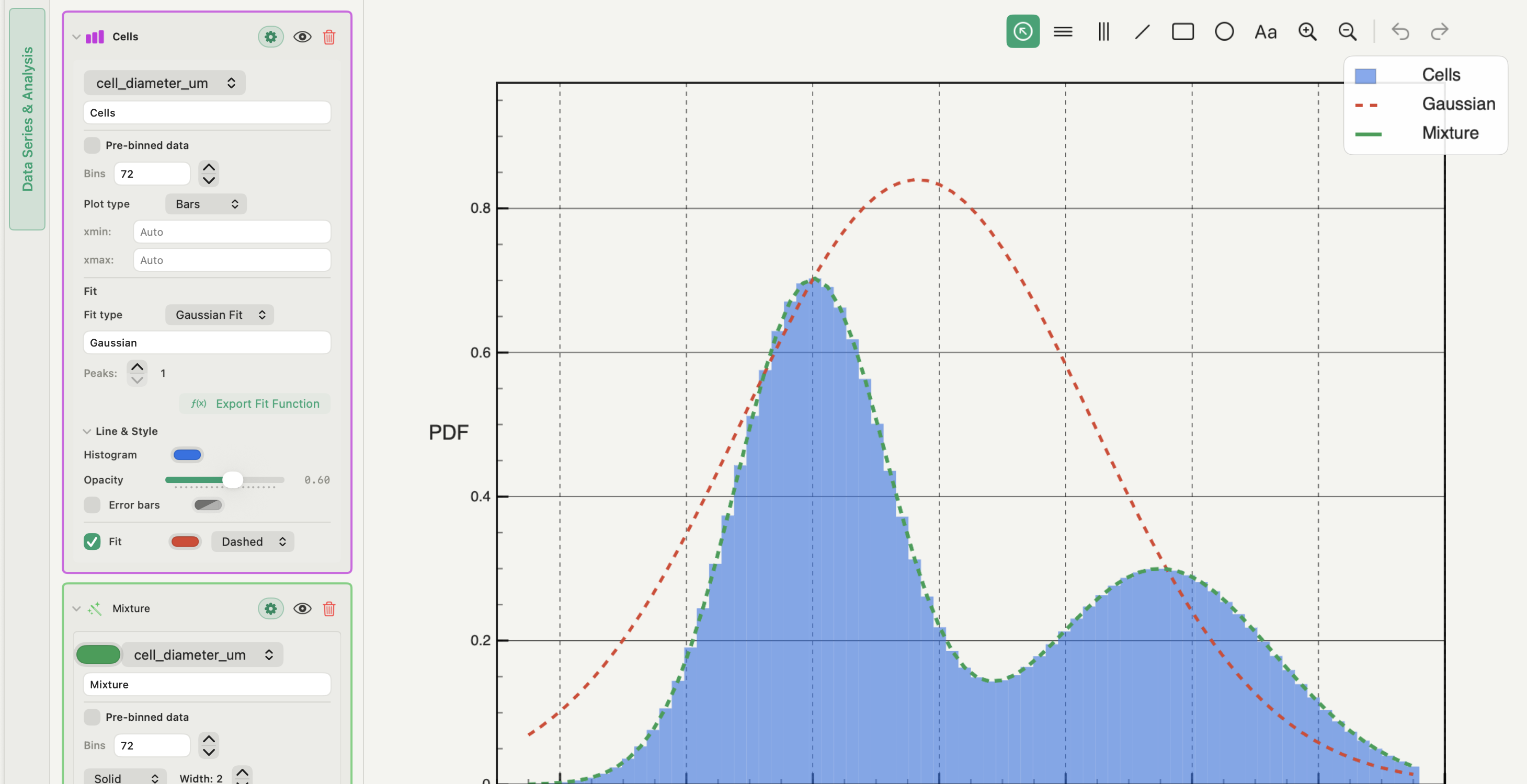
Autoplot's histogram fit is nonlinear least squares on bin centres and densities, with one to three Gaussian components or a predefined or custom formula. It reports each component with parameter errors and R², and the fit can be exported as a reusable function. Log-binned PDFs, power-law fits, CCDF tail fits and an xmin scan cover heavy-tailed data.
More than one kind of plot
Heat maps with rectangular or hexagonal binning and a choice of aggregation, 3D surfaces and scatter plots, and correlation matrices live in the same project as the X&Y plots.
Python when a card is missing
For a model Autoplot does not package, the assistant writes SciPy code, runs it on your Mac inside a working folder and keeps the script. You see the code before it runs. That is a reasonable route for a one-off custom fit, not a replacement for MagicPlot's interactive peak work.
Move one MagicPlot project to Autoplot
- Keep the
.mppzproject and note the MagicPlot version that opens it. - Choose a project that needs something MagicPlot does not do for you, such as a heat map or a tail fit.
- Find the source data as delimited text: the original file you imported into MagicPlot, or the table copied out of it, with column names and units.
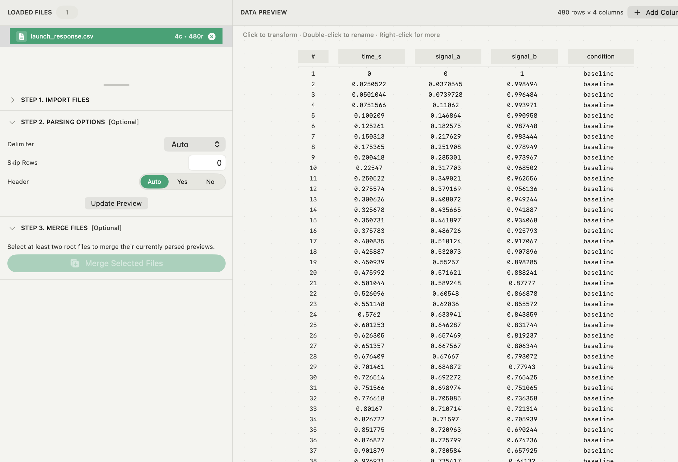
- Import it into Autoplot and check the parser preview: delimiter, header row, row count and missing values.
- Rebuild the plot and run the new analysis. If the result depends on a multipeak model, leave that fit in MagicPlot.
- Where both tools fit the same model, compare parameters, errors, weighting and fit range, then the residuals. Two curves that overlap can still come from different fits.
- Export the deliverable and check its size, fonts and line weights.
The CSV plotting guide covers steps 3 to 5, and how to interpret residual plots covers step 6.
What Autoplot covers, and where it stops
Autoplot needs an Apple silicon Mac (M1 or later) running macOS 15 or later. The free plan, which does not expire, covers X&Y plots, histograms with Gaussian-mixture and custom fits, log-binned distributions and power-law fits. Plus adds heat maps with 2D fits, 3D plots, correlation matrices, Compose, the CCDF card and the xmin diagnostic, and is free for the first 30 days. See the features page and pricing.
It does not open .mppz files, has no interactive multipeak or baseline fitting, and does not run on Windows or Linux, both of which MagicPlot supports. For a wider view of the options, see scientific plotting software for Mac.
Frequently asked questions
| Is MagicPlot available for Mac? | Yes. MagicPlot 3.2 has native downloads for Apple silicon and Intel Macs. |
|---|---|
| Can Autoplot open MagicPlot .mppz files? | No. Import the original data file, or the table copied out of MagicPlot as delimited text, and rebuild the figure in Autoplot. |
| Can Autoplot do multipeak fitting? | Not interactively. Its histogram fit handles up to three Gaussian components on binned data; for spectral peaks, keep MagicPlot or have the assistant write SciPy code for a specific model. |
Sources
Autoplot statements are based on the app's documentation for import, X&Y plots, the histogram fit and the distribution cards, checked on 9 October 2026, and on the features page. MagicPlot's version, platforms, batch processing and export formats come from the MagicPlot site; its project structure from Getting Started; and its Fit Plot, multipeak, baseline, weighting and parameter features from the fitting documentation, all checked on 9 October 2026.