On this page
The bias–variance trade-off of a lower cutoff
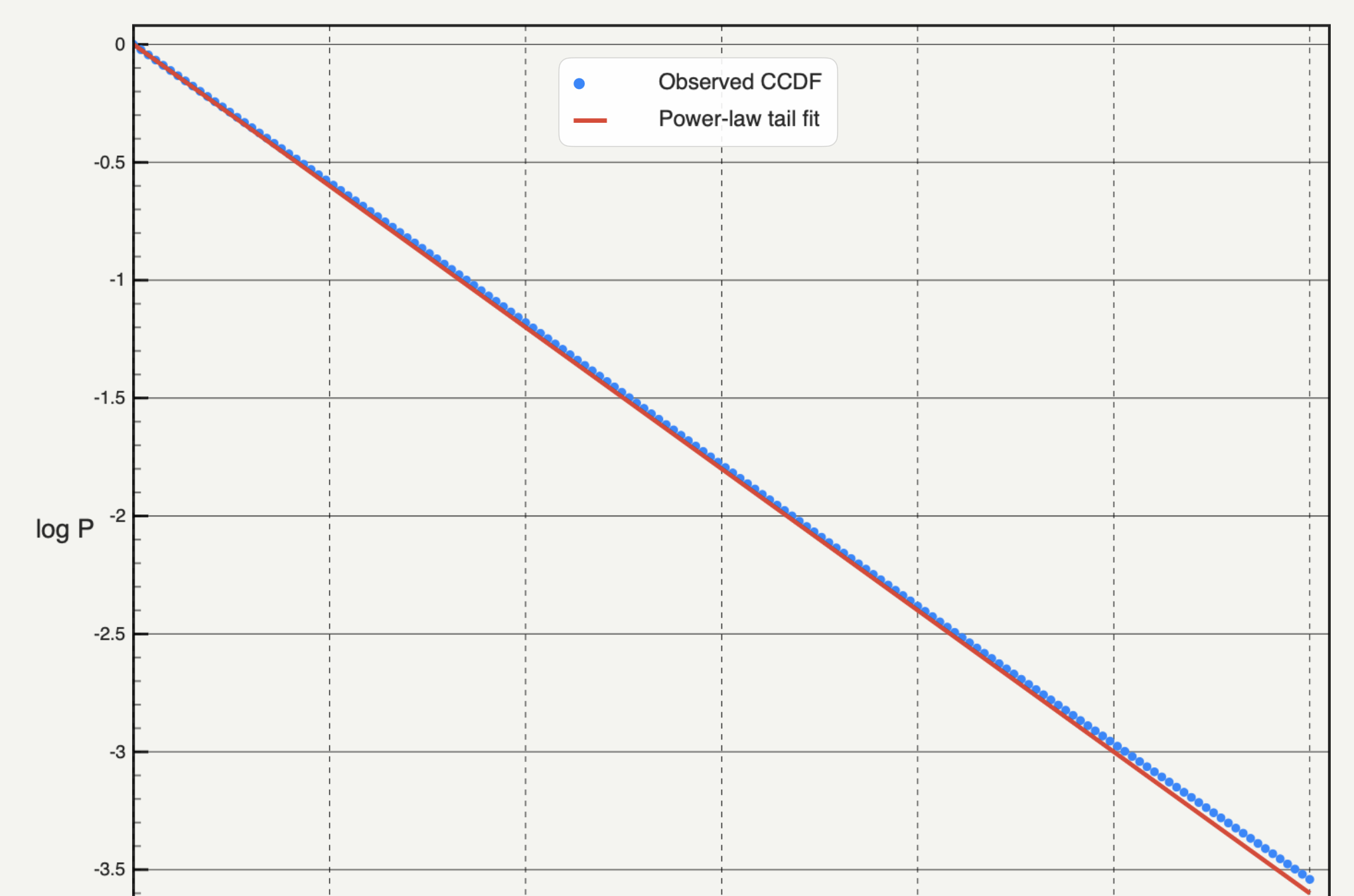
Empirical heavy-tailed quantities rarely follow a power law down to their smallest values. Threshold effects, measurement resolution, or a lognormal-like core typically flatten or round the distribution below some scale, while the power law describes only the upper tail x ≥ xmin.
| Cutoff mistake | Effect on α | How it appears in diagnostics |
|---|---|---|
| xmin set too low | Biased downward (or mixed across regimes) | High KS distance D; visible curvature between data and fit at small x |
| xmin inside scaling plateau | Stable within parameter standard error | Broad shallow basin in D(xmin) with n_tail still well above ~100 |
| xmin set too high | High variance, sensitive to individual extreme values | Sudden drops or jumps in D alongside small n_tail |
This guide focuses on cutoff selection diagnostics and failure modes. For how the chosen cutoff plugs into a binned PDF vs unbinned CCDF workflow and what other evidence a power-law claim needs, see how to fit a power law to data.
How the KS-distance scan picks best xmin
Clauset, Shalizi and Newman's standard procedure scores every distinct observation c in the sorted sample as a trial cutoff:
- Keep the observations x ≥ c and compute the maximum-likelihood power-law exponent α̂(c).
- Evaluate the fitted cumulative distribution function P_c(x) over x ≥ c alongside the empirical CDF S(x).
- Record the Kolmogorov–Smirnov distance
D(c) = max_{x ≥ c} |S(x) − P_c(x)|— the largest vertical gap between the two cumulative curves. - Select
best xminas the candidate cutoff with the smallestD(c).
Even when you expect an exponential roll-off at large values, powerlaw's standard workflow chooses best xmin using the pure power-law KS sweep first, then compares the truncated model above that fixed cutoff. Comparing D directly across different parametric families inside the sweep can reward extra parameters unfairly rather than identifying where scaling begins.
Reading D(xmin) curves: plateaus, spikes and right-edge traps
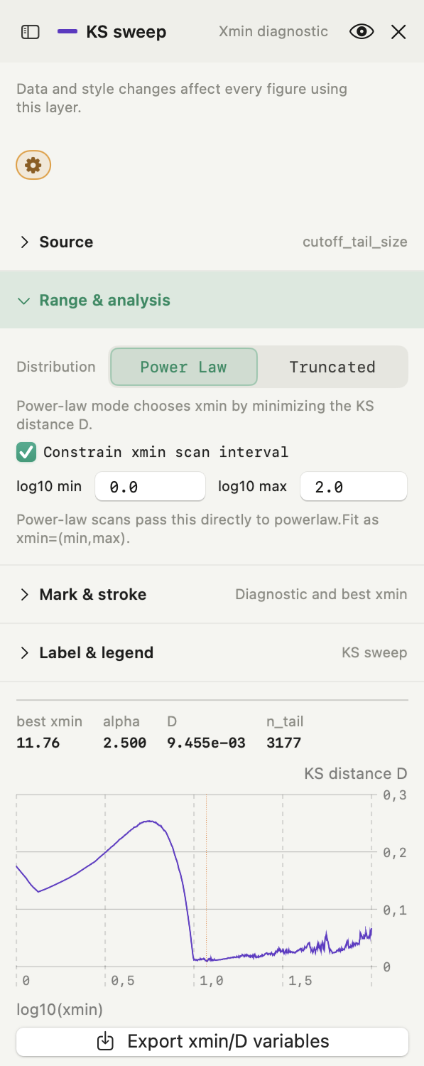
Looking at the single best xmin number without inspecting the D(xmin) curve hides whether the cutoff is well localized or accidental.
| Shape of D(xmin) | What it indicates | Practical response |
|---|---|---|
| Broad flat valley spanning ~1 decade | Tail matches power law across a clear range; small D shifts barely change quality | Consider picking near the lower edge of the flat valley if α is already stable, to retain larger n_tail |
Sharp dip at high xmin with tiny n_tail | Small-sample noise makes an empirical step fit closely by accident | Cap the upper search boundary (log₁₀ max) so candidates with too few points cannot win |
| Monotonic drop across the entire range | True distribution likely curves continuously (e.g. lognormal) with no pure tail regime | Compare alternatives directly via power law vs lognormal instead of pushing xmin higher |
| Sawtooth steps or multiple local dips | Rounded values, ties, or secondary regimes | Plot the raw empirical CCDF first to inspect staircases or measurement resolution |
Upper cutoffs and sensitivity checks before trusting best xmin
- Set a hard upper cutoff (xmax) before scanning if physical finite size, sensor saturation, or collection windows cap large values. Without
xmaxsupplied ahead of time, the pure power-law KS scan sees the upper drop-off as a bad fit and pushesxminartificially rightward. - Plot α(xmin) and n_tail beside D(xmin). Export the sweep curve or refit at half and twice
best xmin: if α drifts steadily as xmin grows, the minimum ofDmay just be trading one curved region for another. - Check whether an exponential tail explains the same range better. Run a truncated comparison above
best xmin; when truncation explains the upper bend cleanly, forcing a higherxminon a pure power law wastes data. - Do not confuse D with a p-value. A small
D(such as0.02) simply identifies the closest cutoff within the assumed power-law family; it does not test whether synthetic power-law samples produce deviations as large as yours.
Xmin diagnostics in Autoplot
Autoplot's Xmin Diagnostic card (Run Analysis → Xmin Diagnostic, Plus) requires at least 50 finite positive observations and runs powerlaw.Fit locally through Python.
- Power Law mode: sweeps candidate cutoffs, plots
Dvslog₁₀(xmin), marksbest xmin, and reportsbest xmin(in natural units),alpha,Dandn_tail. - Truncated mode: selects
best xminvia the same power-law KS sweep, then fitspower_lawandtruncated_power_lawabove that cutoff and runsdistribution_compare('power_law', 'truncated_power_law'), reportingalpha_tr,alpha_pl,lambda,Randp. - Interval and upper-cutoff controls: toggle Constrain xmin scan interval (
log₁₀ min,log₁₀ max) to avoid sparse high-tail artifacts, and in Truncated mode toggle Use hard upper cutoff (log₁₀ xmax) to passxmaxbefore the KS scan. - Export xmin/D variables: saves the candidate
xminandDarrays as reusable workspace variables so you can overlay sensitivity plots or inspect plateaus at full scale.
Note that UI fields on the card (log₁₀ min, log₁₀ max, log₁₀ xmax) take base-10 logarithms, whereas best xmin in Results is printed in natural units. The card does not scan D(xmin) under a lognormal model or run Clauset, Shalizi and Newman's Monte Carlo goodness-of-fit test; run those checks via Python or Autoplot's assistant when preparing a formal publication claim. See features and pricing.
Frequently asked questions
| Why can minimizing KS distance pick an unreasonably high xmin? | When very few observations remain above a large trial cutoff, a short empirical tail has fewer chances to deviate strongly from the fitted line, or ties create low-D pockets. Constraining the upper scan limit keeps at least ~50–100 observations in the tail. |
|---|---|
| Should I constrain xmin before running the scan? | Only with a clear reason: excluding noisy micro-values below instrument resolution or preventing tiny-sample spikes near the maximum. Inspect the unconstrained D(xmin) curve first so your constraints stay documented and honest. |
| Why does Autoplot's Truncated mode still find xmin using Power Law? | Following the powerlaw library workflow, selecting xmin under a single-parameter power law isolates where scaling begins, and the nested likelihood-ratio test (R and p) then compares pure vs truncated power laws over that identical tail sample. |
Sources
Autoplot behaviour comes from the app's Python engine (compute_xmin_vs_ks in math_logic.py) and XminDiagnosticCardEditor, checked on 14 November 2026, plus the features page. Clauset, Shalizi and Newman, Power-law distributions in empirical data, defines the KS-minimization cutoff estimator (Section 3.3). The powerlaw package implements Fit and xmin_fitting_results.