On this page
Why a lognormal tail mimics a power law
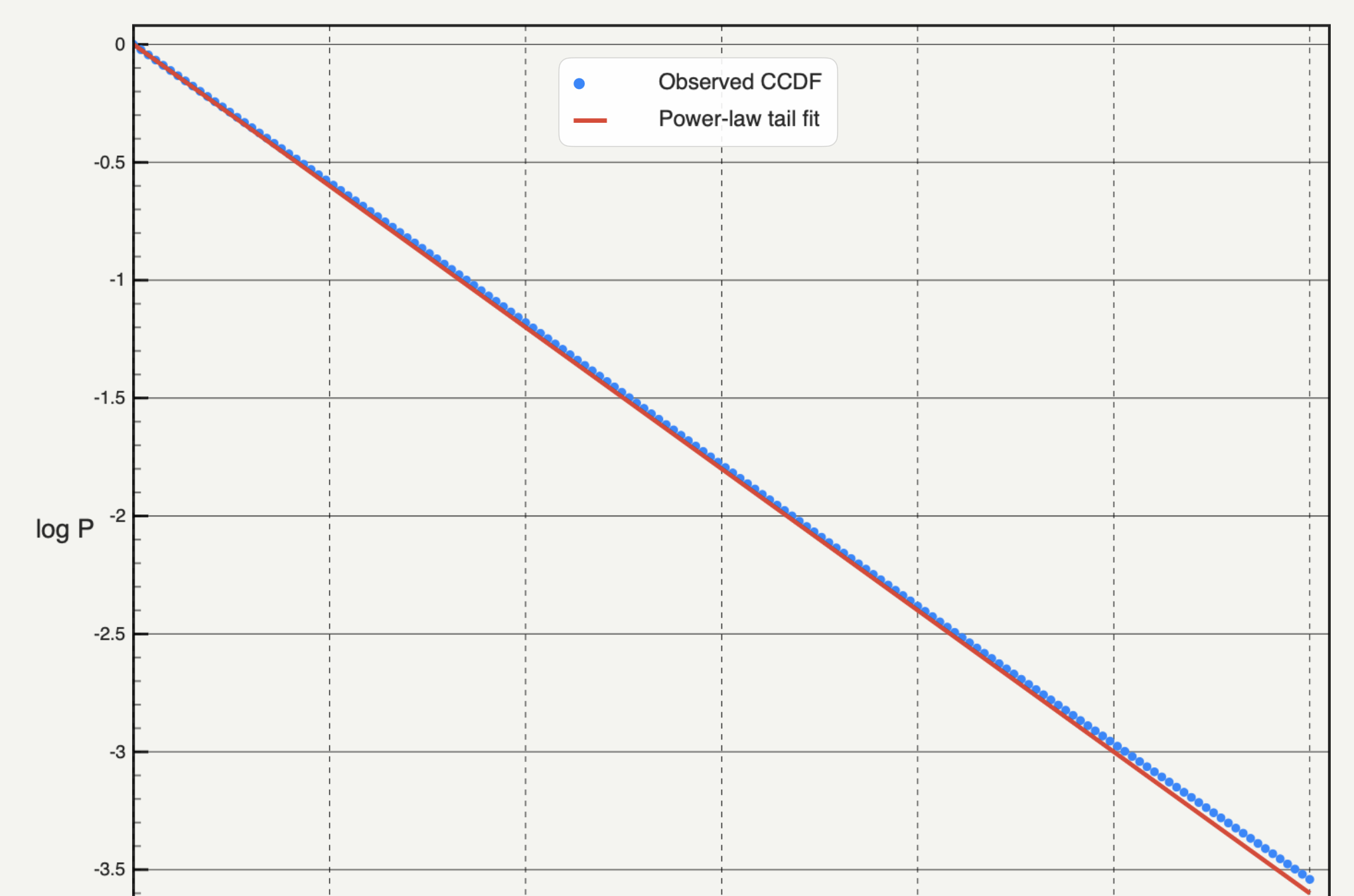
On a log–log complementary cumulative distribution (CCDF), a pure power law is a straight line with slope −(α − 1). A lognormal density has a quadratic term in ln x, so its log–log curve bends downward continuously—but when σ is large enough, that curvature is subtle over a typical three-decade empirical sample.
| Distribution | Generating mechanism | Log–log CCDF shape | Fitted tail parameters |
|---|---|---|---|
| Power law | Scale-free growth or criticality | Straight line above xmin | α, xmin |
| Truncated power law | Scale-free with finite-size cutoff | Straight middle, exponential roll-off | α, λ, xmin |
| Lognormal | Multiplicative positive factors | Gentle downward curve over decades | μ, σ, xmin |
The lower right of an empirical CCDF is where lognormal curvature shows most clearly, and also where the fewest observations live. When a sample holds fewer than a few hundred points in the tail, random fluctuations in the top decade easily mask real curvature or create apparent bends. See how to make a CCDF plot for how sample size controls tail depth.
Compare both models above the same xmin
Likelihoods are only comparable when both candidate distributions explain the exact same subset of observations, normalized on the same domain. Changing xmin changes which points enter the likelihood, making log-likelihood values incomparable across different cutoffs.
- Fix a candidate lower cutoff xmin from raw positive observations—for example via a Kolmogorov–Smirnov distance scan in how to choose xmin for a power law—and record the tail count n_tail (x ≥ xmin).
- Fit both a power law and a lognormal on those raw observations x ≥ xmin by maximum likelihood (continuous or discrete, matching your data type). Never compare a binned least-squares PDF R² against an unbinned CCDF likelihood.
- Compute the log-likelihood ratio R = ln L_power_law − ln L_alternative and its normalized p-value across the individual observations in that tail.
- Repeat the comparison at neighbouring values of xmin (and any physical upper bound xmax) to verify that the sign and significance do not flip with a minor boundary tweak.
In Python's powerlaw package, fit = powerlaw.Fit(data) followed by R, p = fit.distribution_compare('power_law', 'lognormal') implements this exact normalized comparison using Vuong's closeness test for non-nested distributions.
How to read R, p and a non-significant result
Because the sign of R gives the direction and p tests whether individual per-point log-likelihood differences could arise from sampling noise, neither number is complete on its own.
| Result | Interpretation | Honest conclusion |
|---|---|---|
| R > 0 and p < 0.1 | Power law gives higher likelihood than lognormal beyond chance noise | Power law is favored over lognormal, subject to a goodness-of-fit test |
| R < 0 and p < 0.1 | Lognormal fits the tail meaningfully better than a pure power law | Reject pure power law in favor of lognormal or another curved model |
| p ≥ 0.1 (any R) | Log-likelihood variance overlaps zero across observations | Inconclusive: the dataset cannot distinguish power law from lognormal |
When p ≥ 0.1, do not report the sign of R as mild support for a power law. In empirical data with fewer than ~1,000 tail observations, inconclusive tests between lognormal and truncated power law are common: both capture gentle downward curvature, and a larger sample is often the only way to tell them apart.
Pure vs truncated power law is nested
A pure power law is a special case of an exponentially truncated power law (λ = 0). Because one model nests inside the other, likelihood ratio R has a fixed direction and its p-value follows a chi-square test rather than Vuong's two-sided normal test. In real systems bounded by detector range or system size, truncated_power_law frequently outperforms both pure power_law and lognormal once the cutoff reaches the upper bend.
What Autoplot compares in cards and what needs Python
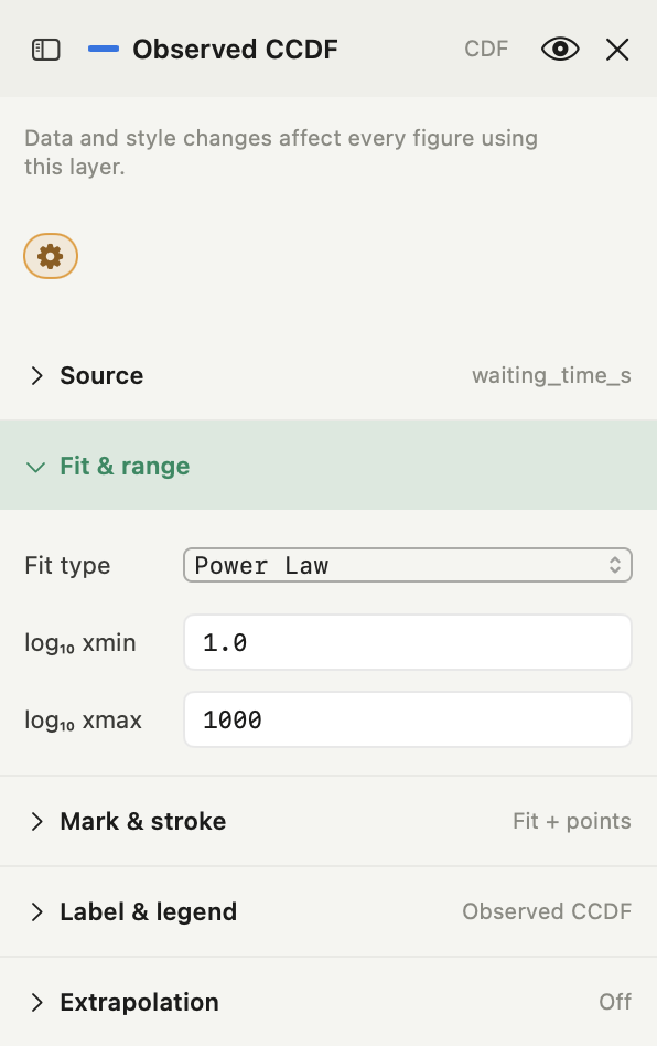
Autoplot's Observed CCDF card (Run Analysis → Log-Space CCDF Fit, Plus) fits four models individually to raw positive values above your chosen log₁₀ xmin (and optional log₁₀ xmax) via continuous maximum likelihood through the powerlaw library: Power Law (reporting alpha), Truncated PL (alpha, Lambda), Log-Normal (mu, sigma), and Stretched Exponential (beta, Lambda). Every fit uses the full filtered tail without binning and reports KS distance D, n_tail and full-sample normalization. You can add separate Observed CCDF cards on one figure with the same bounds to overlay Power Law and Log-Normal curves and compare their D values visually.
Autoplot's Xmin Diagnostic card (Plus), in Truncated mode, automatically runs fit.distribution_compare('power_law', 'truncated_power_law') at the KS-selected best xmin and reports alpha_pl, alpha_tr, lambda, R and p directly in the card.
What neither card runs: Autoplot does not have a built-in button that outputs Vuong's R and p between Power Law and Log-Normal, nor does it run Clauset, Shalizi and Newman's simulation-based goodness-of-fit p-value. To run fit.distribution_compare('power_law', 'lognormal') or bootstrap p-values, run Python locally or ask Autoplot's assistant to generate and run a powerlaw comparison script in your project workspace (read the saved script before relying on it). See the features page and power-law fitting guide for card capabilities.
Frequently asked questions
| Can I use R² from a log–log plot to choose power law over lognormal? | No. Least-squares R² measures how tightly binned or cumulative points sit around a line and stays high even when an unbinned sample follows a broad lognormal curve. Use maximum-likelihood ratio testing on the raw tail values instead. |
|---|---|
| What does a large p-value (p ≥ 0.1) mean in a likelihood-ratio comparison? | It means the observed log-likelihood difference between the two models is indistinguishable from random sample variation. Report that the data are consistent with both distributions rather than claiming the preferred model by the sign of R alone. |
| Why does Autoplot fit Log-Normal in the CCDF card without printing an R or p value? | The Observed CCDF card evaluates one selected family at a time (Power Law, Truncated PL, Log-Normal, or Stretched Exponential) and reports its parameters and KS distance D. Only the Xmin Diagnostic card's Truncated mode runs a built-in likelihood-ratio test (power_law vs truncated_power_law). |
Sources
Autoplot behaviour comes from the shipped CCDF and Xmin Python implementations (compute_cdf and compute_xmin_vs_ks) and card inspectors, checked on 14 November 2026, plus the features page. Clauset, Shalizi and Newman, Power-law distributions in empirical data, defines the maximum-likelihood ratio test (Section 4.2, based on Vuong's test) and non-nested vs nested comparison rules. Alstott, Bullmore and Plenz, powerlaw, documents distribution_compare and model definitions.