
On this page
What the finite-size scaling ansatz assumes
When avalanches, fracture bursts, or critical clusters grow inside a finite domain of linear size , large events cannot exceed a characteristic cutoff scale . Following Salman, Ahadi, and Truskinovsky (2026), Eq. 43 writes the size distribution at size as
Here is the positive event observable (such as stress drop or dissipated energy ), is the power-law decay exponent ( for stress drops, for energy drops; denoted in Autoplot's search UI), is the fractal cutoff dimension controlling how fast the upper cutoff grows with system size , and is the dimensionless scaling function describing both the critical power-law plateau and the finite-size rollover.
Before running a multi-size collapse, establish on individual sizes that a heavy tail actually exists and where lower non-scaling structure ends. See log binning for width-normalized density estimation across orders of magnitude, and how to choose xmin for a power law for separating small-scale discretization or threshold effects from the scaling regime.
How data collapse minimizes overlap variance in log-coordinates
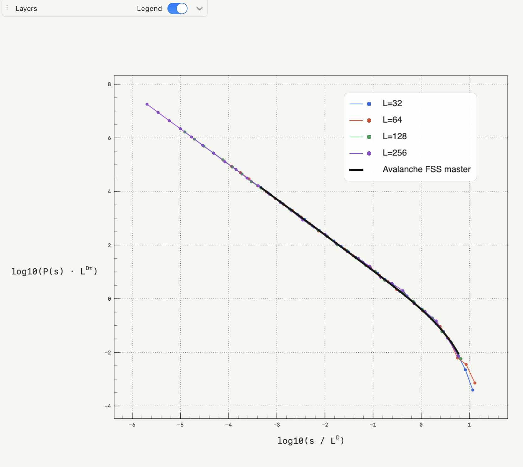
Data collapse turns visual curve alignment into an explicit variance minimization over log-rescaled densities (Salman, Ahadi, and Truskinovsky, 2026, Eqs. 44–50):
- Bin raw samples on logarithmic grids: for each dataset with linear system size , restrict positive observations to , build log-spaced bin edges, evaluate geometric bin centers, and normalize bin counts by to obtain probability densities .
- Rescale into collapsed log10 coordinates: for a candidate pair , map each non-empty bin center and density to and
- Find the strict common overlap : set and , linearly interpolate each curve onto a uniform grid spanning (for example 80 points), and retain the valid grid subset where all curves are defined inside their measured bounds.
- Minimize cross-size variance : compute the average variance across all curves at each valid grid point : where is the cross-size mean at .
- Select the best pair on the search grid: evaluate across the search grid (optionally narrowing onto a local fine grid around the best coarse point) to find the parameters that minimize variance.
- Estimate operational errors from the profile: project onto 1D minimum-variance profiles along and , fit a local quadratic around the minimum grid point, and take the half-width where the fitted variance doubles to :
Reading collapse diagnostics and spotting boundary traps
A clean numerical minimum does not automatically mean the data obeys finite-size scaling. Always read the summary table, search bounds, and overlap together:
| Diagnostic signal | What it tells you | Action to take |
|---|---|---|
Optimum hits a search limit (τ min/max or D min/max) | True minimum lies outside your search box or slopes monotonically without a local valley | Widen search bounds and confirm a true interior minimum appears |
No stable overlap found or very short | Curves barely overlap in under min overlap or aggressive per-size cutoffs | Relax unnecessary xmin/xmax cutoffs or widen spacing gradually rather than dropping intermediate sizes |
| Crisp collapse for sizes only | Two decaying curves can align under many tradeoffs across short intervals | Add at least one or two intermediate or larger system sizes so both slope and finite-size rollover lock down |
| agrees across regimes while jumps sharply | Bulk power-law scaling persists while event geometry changes | Inspect spatial morphology or cutoff structure separately; exponent similarity alone does not imply identical geometry |
In crystal plasticity simulations by Salman, Ahadi, and Truskinovsky (2026), preyield and postyield dissipated energy bursts illustrate that fourth row directly: energy exponents stay close ( preyield vs postyield across ~5–6 decades) even as the cutoff fractal dimension jumps from nearly point-like localized events () to system-spanning branched bands (), while stress drops shift in both exponent ( to ) and dimension ( to ).
Why an attractive collapse is not proof of universality
Visual curve collapse is a consistency check, not a hypothesis test or proof of universality. Three guardrails keep a finite-size scaling figure scientifically defensible:
- Read quality as an overlap variance, not a p-value:
quality() is the mean variance across interpolated log densities, not a chi-square statistic or statistical goodness-of-fit test, and depends ondefault bins,min overlap,interp pts, and cutoffs. - Test sensitivity to cutoffs and bin count: vary
default bins(for example 20 vs 30 vs 40) and re-check small- discretization cutoffs (raw log10 xmin) to verify fitted remain stable. - Check single-size fits alongside the collapse: confirm that individual system sizes support a heavy tail rather than curving continuously everywhere using power law vs lognormal tails or a binned vs CCDF check in how to fit a power law to data.
Running FSS Collapse in Autoplot
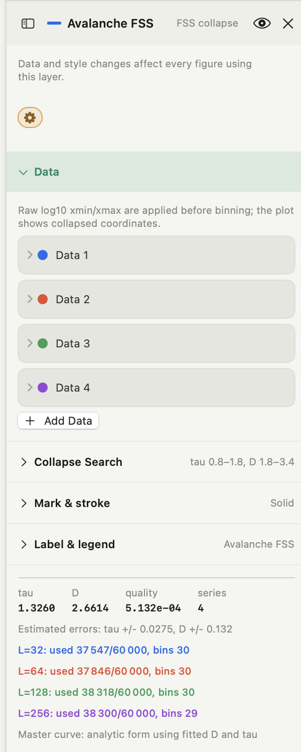
Autoplot's FSS Collapse layer (Run Analysis → FSS Collapse in an X&Y Plot figure, Plus) implements the variance-minimization collapse of Salman, Ahadi, and Truskinovsky (2026) locally on raw positive sample columns without requiring you to pre-bin files outside the app:
- Size-indexed inputs (Data): use
+ Add Datato add two or more positive numeric columns (>= 5points and>= 3non-empty bins each), assign each row its linear system size , and optionally enter per-rowraw log10 xminorraw log10 xmaxcutoffs anddefault bins(default 30, clamped>= 3). Cutoffs are converted from base-10 logarithms () before binning; the figure itself renders collapsed coordinates. - Coarse-to-fine search (Collapse Search): set bounds and resolution (
τ min/max/steps,D min/max/steps), toggleFine search around best grid point(fine steps), adjustinterp pts(default 80) andmin overlap(default 0.5 decades), and click the orange gear button to compute or rerun. - Outputs and warnings (Mark & stroke, card summary, Figure Inspector → Results): Autoplot plots every collapsed series alongside an optional
mastercurve (fitted analytic form using and , falling back to the cross-size mean curve if the weighted analytic fit fails), prints scalar , ,quality(), quadratic profileEstimated errors, and per- used counts/bins, and surfaces boundary ( or on search limits) or overlap (No stable overlap found) warnings. Autoplot does not plot the 2D surface or 1D profile curves directly.
Frequently asked questions
| Should I pass raw event values or pre-binned histogram heights into FSS Collapse? | Pass raw positive event columns (one variable per system size ), not already binned histogram counts or densities. Autoplot applies each row's raw log10 xmin and raw log10 xmax cutoffs first and constructs width-normalized logarithmic probability densities internally before searching . |
|---|---|
| What does Autoplot's quality metric mean, and can I compare it across papers? | quality is the mean cross-size variance of interpolated values over the shared overlap grid . Smaller indicates tighter overlap for fixed binning, overlap settings, and sample size , not an absolute p-value—only compare across runs or parameter settings that share the same binning, cutoffs, and overlap window. |
| Why did FSS Collapse warn that best τ or D is on the search boundary? | If optimal equals τ min/τ max or optimal equals D min/D max, the true variance minimum likely lies outside your configured interval—or decreases monotonically across the search box without an interior valley. Widen the search bounds and rerun so the minimum is strictly bracketed inside the grid. |
| How does Autoplot compute Estimated errors for τ and D? | Autoplot projects the grid quality surface onto 1D minimum profiles around the best grid point, fits a local quadratic polynomial , and prints (the half-width where the fitted variance doubles to ). Because Autoplot outputs these scalar widths without plotting the landscape itself, check stability across nearby binning and cutoff choices as well. |
| What happens if one system size covers a much narrower x-range than the others? | Because takes the strict intersection across every active series, a single poorly populated or heavily truncated curve shrinks the valid overlap domain . If drops below min overlap, Autoplot emits "No stable overlap found; relax cutoffs or minimum overlap." Inspect per- used/total counts and adjust cutoffs or exclude incomplete trial runs intentionally. |
Sources
Finite-size scaling equations, the variance-minimization quality score , operational profile error estimation, and crystal-plasticity empirical contrasts are adapted from O. U. Salman, A. Ahadi, and L. Truskinovsky, "Self-induced marginality in plastically deformed crystals," *Physical Review Materials* 10, 103611 (2026), DOI `10.1103/3rwf-d3yx` (published under CC BY 4.0). Autoplot UI labels, logarithmic binning rules, quality, and profile_sigma error calculation come directly from Autoplot's Python engine (compute_fss_collapse in math_logic.py) and FSSCollapseCardEditor, verified on 15 November 2026.