
On this page
When a power-law scaling relation applies
Unlike univariate tail analysis, which models how frequently events of size occur (), a scaling relation describes how one positive observable scales conditionally with a paired observable measured on the same event:
Taking base-10 logarithms turns the power law into an affine relation with slope and intercept :
Across scientific fields, power-law scaling relations capture how two positive observables co-vary across decades—from allometric metabolic rate versus body mass in biology (West, Brown, and Enquist, 1997) to avalanche size, energy, and duration in crackling-noise systems (Sethna, Dahmen, and Myers, 2001). Together with finite-size scaling and data collapse, scaling relations give complementary checks: data collapse tests whether size-indexed distributions share one universal scaling function, whereas a scaling relation directly quantifies the power-law dependence between paired observables within events.
Notice also how the error structure affects regression choice: Xiao et al. (2011) show that ordinary least squares in coordinates is well matched when fluctuations around are multiplicative (lognormal scatter in at fixed ), whereas arithmetic errors require nonlinear regression on untransformed variables in how to fit a curve to data. Always verify that both columns span two to three decades, remain strictly positive where scaling holds, and stay row-aligned event by event.
How log-log regression weights raw clouds vs log-binned means
Autoplot's Scaling Relation engine turns paired observables into an ordinary least-squares fit in base-10 log coordinates:
- Filter positive row-aligned pairs: keep only rows where both and , then transform to log coordinates and .
- Optionally aggregate into uniform bins: when binning is enabled (
Do Binning), divide into equal-width intervals . For each non-empty bin, compute the linear midpoint and conditional mean log response along with the within-bin spread . Unlike density estimates in log binning, conditional means are not divided by bin width because is an event observable rather than a probability density. - Apply optional range cutoffs after binning: if lower or upper bounds (
log₁₀ sMin,log₁₀ sMax) are provided, filter the active fit points (non-empty bin centers when binning is active, or raw pairs otherwise) to , requiring at least points. - Fit unweighted OLS and slope error: minimize over the retained points to compute slope , prefactor , coefficient of determination in space, and (for ) the OLS standard error of the slope: where and .
Choosing between raw pairs, log-binned means, and range cutoffs
Because heavy-tailed observables pack orders of magnitude more points at small than at large , raw regression and binned-mean regression answer slightly different weighting questions:
| Regression setup | What drives the slope | Watch out for |
|---|---|---|
Raw positive pairs (Binning unchecked) | Every observed pair carries weight | When follows a heavy tail, dense low- noise dominates and large rare events barely move |
Equal-width bin means (Binning checked) | Every non-empty bin carries weight | Sparse upper bins containing only 1–2 events get equal leverage to dense lower bins |
Narrower log₁₀ sMin / log₁₀ sMax window | Isolates an intermediate inertial range free of threshold rolloff | Over-trimming noisy ends manufactures artificially clean lines; report bounds alongside |
| Comparing raw vs binned fits on the same data | Checks whether scatter is symmetric around a single global slope | Large divergence between raw and binned flags curvature, heteroscedastic spread, or asymmetric tails |
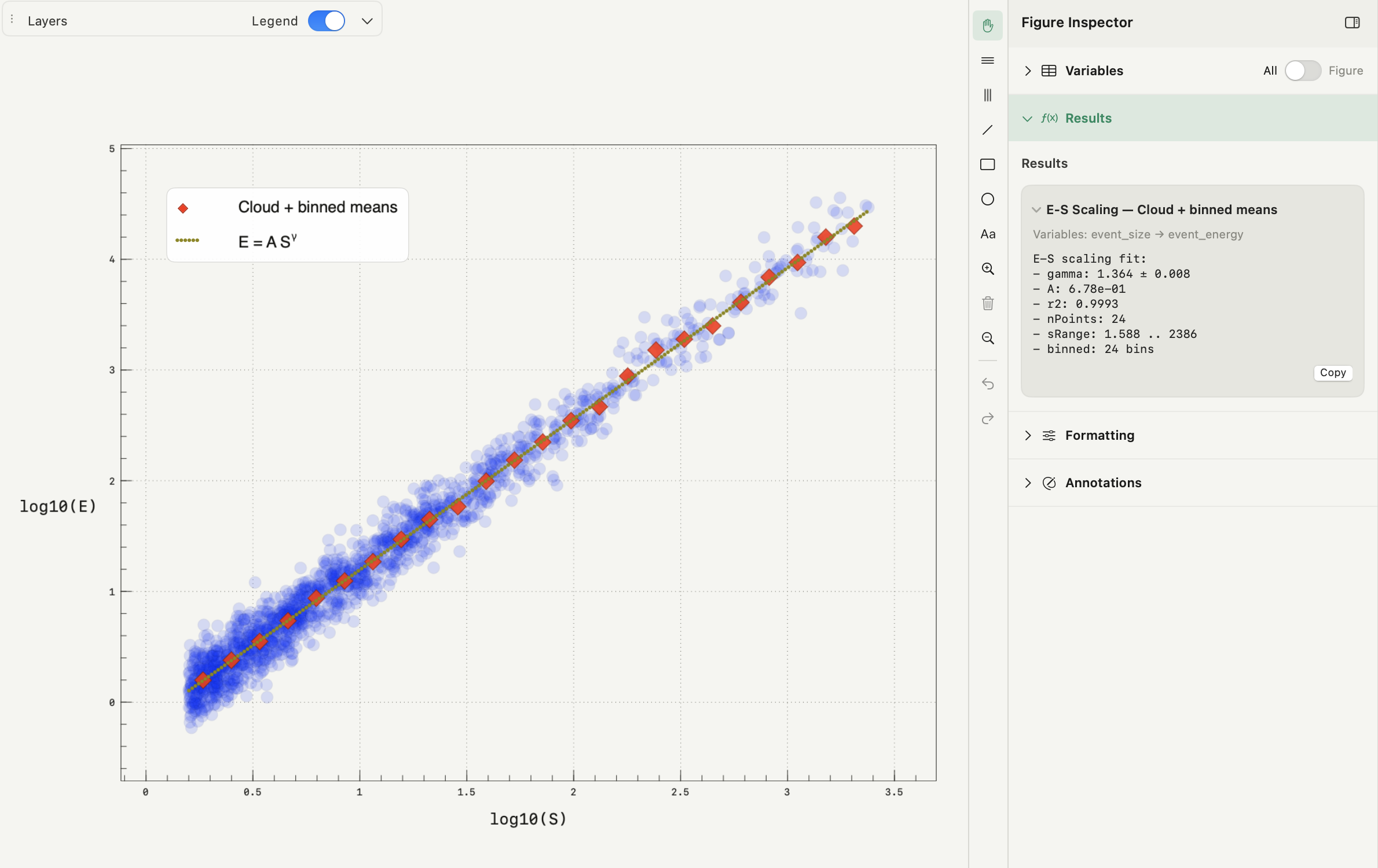
On a heavy-tailed synthetic ensemble of 1,500 paired events (, , multiplicative scatter ) in Autoplot, both methods recover the underlying slope consistently ( raw vs across 24 log bins), while raw point scatter keeps unbinned whereas bin-averaging lifts binned to 0.9993.
What log-log R² does and does not prove
A linear regression line across three or more orders of magnitude will look impressive under even when a true physical power law fails. Three checks keep a scaling exponent defensible:
- Do not confuse log-space with a scaling-law proof:
r2is evaluated directly on residuals—and on bin means when binning is checked—so averaging out within-bin variance can push above 0.99 even when raw points scatter widely or curve gently. - Audit systematic curvature across decades: compare binned means against the fitted line visually and inspect local deviations as described in how to interpret residual plots. Consistent S-shaped bowing across bins points to crossover scales or non-power-law behavior rather than random error.
- Run cutoff and bin-count sensitivity sweeps: re-run with nearby
Binscounts (for example16,24,36) and plausiblelog₁₀ sMin/log₁₀ sMaxboundaries, and verify univariate tail behavior first using how to fit a power law to data. Note also that log-log OLS optimizes errors in assuming exact ; errors-in-variables attenuation occurs if itself carries large measurement noise.
Running Scaling Relation in Autoplot
Autoplot's Scaling Relation layer (Run Analysis → Scaling Relation in an X&Y Plot figure, Plus) computes row filtering, optional binning, and log–log regression locally on your Mac:
- Paired variables (Source): select row-aligned numeric columns
SandE(>= 2paired rows; rows with or are dropped before taking ). - Binning and domain bounds (Range & binning): toggle
Binning, setBins(1–1000), and optionally restrict the fit window in base-10 log units usinglog₁₀ sMinandlog₁₀ sMax(applied after binning, falling back to raw pairs if<= 1non-empty bin exists). - Plot styling and results (Mark & stroke, Figure Inspector → Results): customize the fit line (
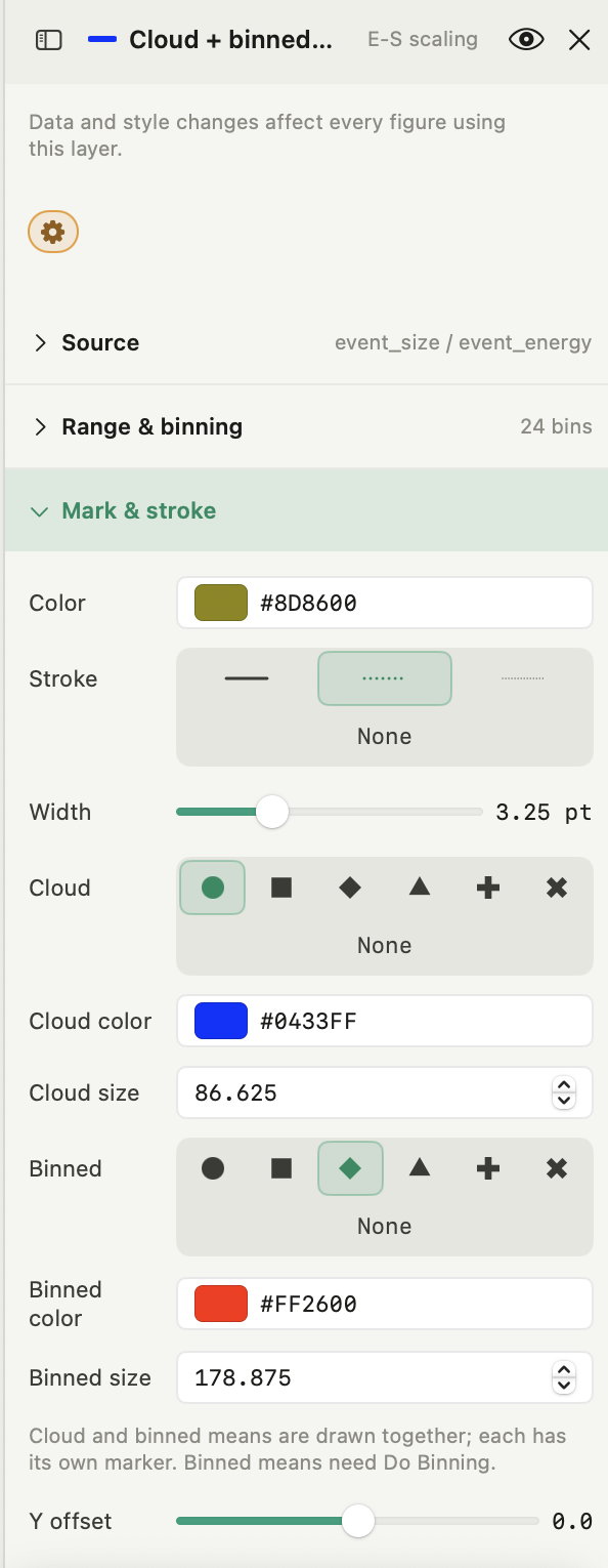
Color,Stroke,Width) independently fromCloud(display cloud sampled up to5,000positive raw rows) andBinned(Cloud color/sizevsBinned color/size), click the orange gear button, and inspectgamma,A,r2,nPoints,sRange, andbinnedcount inFigure Inspector → Results(E‑S Scaling). Autoplot computes OLS log-spaceR²and slope standard error directly; run custom weighted fits or residual normality diagnostics separately if needed.
Frequently asked questions
| Why do unbinned and log-binned fits give different γ or R² on the same dataset? | Raw OLS weights every (S, E) row equally, so a heavily skewed sample size distribution concentrates leverage near small . Checking Binning averages inside uniform bins first so each decade contributes evenly, and removing within-bin scatter increases binned relative to raw-cloud . |
|---|---|
| Should I enter natural numbers or base-10 logarithms in log₁₀ sMin and log₁₀ sMax? | Enter base-10 logarithms of your variable (for example 1.0 for , 3.0 for ). Autoplot converts both bounds via and filters the binned centers (or raw points when unbinned) to lie inside [sMin, sMax]. |
| What happens if one of my variables contains zeros or negative values? | Scaling Relation keeps only paired rows where both and ; zero or negative entries are omitted before taking . If zeros or negative values carry signal rather than invalid rows, fit on linear axes in how to fit a curve to data instead. |
| Does Autoplot plot residual diagnostics or curvature tests for Scaling Relation automatically? | No. Autoplot displays the raw cloud, optional binned means, fitted power-law line, and scalar summary metrics (gamma SE, A, log-space r2, nPoints, sRange, binned count) under Figure Inspector → Results. Check curvature visually against the plotted binned means and run formal weighted or residual checks across varying Bins and log₁₀ sMin/sMax cutoffs. |
Sources
Algorithm details (es_scaling_fit positive filtering, left-closed right-open bins, post-binning range filter, manual OLS slope standard error, and log-space r2) and UI labels (Source, Range & binning, Mark & stroke, Label & legend, E‑S Scaling results block) were verified directly against Autoplot's Python engine (math_logic.py), ESScalingFitCardEditor, and live Autoplot 2.1.1 captures on 18 November 2026. Cross-disciplinary scaling examples and log-transformation regression trade-offs draw on G. B. West, J. H. Brown, and B. J. Enquist, "A General Model for the Origin of Allometric Scaling Laws in Biology," *Science* 276(5309), 122–126 (1997), DOI `10.1126/science.276.5309.122`; J. P. Sethna, K. A. Dahmen, and C. R. Myers, "Crackling noise," *Nature* 410, 242–250 (2001), DOI `10.1038/35065675`; and X. Xiao, E. P. White, M. B. Hooten, and S. L. Durham, "On the use of log-transformation vs. nonlinear regression for analyzing biological power laws," *Ecology* (2011), DOI `10.1890/11-0538.1`.